Tutorial 1 : Opening a window
- Introduction
- Prerequisites
- Forget Everything
- Building the tutorials
- Running the tutorials
- How to follow these tutorials
- Opening a window
Introduction
Welcome to the first tutorial !
Before jumping into OpenGL, you will first learn how to build the code that goes with each tutorial, how to run it, and most importantly, how to play with the code yourself.
Prerequisites
No special prerequisite is needed to follow these tutorials. Experience with any programming langage ( C, Java, Lisp, Javascript, whatever ) is better to fully understand the code, but not needed; it will merely be more complicated to learn two things at the same time.
All tutorials are written in “Easy C++” : Lots of effort has been made to make the code as simple as possible. No templates, no classes, no pointers. This way, you will be able to understand everything even if you only know Java.
Forget Everything
You don’t have to know anything, but you have to forget everything you know about OpenGL. If you know about something that looks like glBegin(), forget it. Here you will learn modern OpenGL (OpenGL 3 and 4) , and many online tutorials teach “old” OpenGL (OpenGL 1 and 2). So forget everything you might know before your brain melts from the mix.
Building the tutorials
All tutorials can be built on Windows, Linux and Mac. For all these platforms, the procedure is roughly the same :
- Update your drivers !! doooo it. You’ve been warned.
- Download a compiler, if you don’t already have one.
- Install CMake
- Download the source code of the tutorials
- Generate a project using CMake
- Build the project using your compiler
- Play with the samples !
Detailed procedures will now be given for each platform. Adaptations may be required. If unsure, read the instruction for Windows and try to adapt them.
Building on Windows
- Updating your drivers should be easy. Just go to NVIDIA’s or AMD’s website and download the drivers. If unsure about your GPU model : Control Panel -> System and Security -> System -> Device Manager -> Display adapter. If you have an integrated Intel GPU, drivers are usually provided by your OEM (Dell, HP, …).
- We suggest using Visual Studio 2017 Express for Desktop as a compiler. You can download it for free here. MAKE SURE YOU CHOOSE CUSTOM INSTALLATION AND CHECK C++. If you prefer using MinGW, we recommend using Qt Creator. Install whichever you want. Subsequent steps will be explained with Visual Studio, but should be similar with any other IDE.
- Download CMake from here and install it
- Download the source code and unzip it, for instance in C:\Users\XYZ\Projects\OpenGLTutorials\ .
-
Launch CMake. In the first line, navigate to the unzipped folder. If unsure, choose the folder that contains the CMakeLists.txt file. In the second line, enter where you want all the compiler’s stuff to live. For instance, you can choose C:\Users\XYZ\Projects\OpenGLTutorials-build-Visual2017-64bits\, or C:\Users\XYZ\Projects\OpenGLTutorials\build\Visual2017-32bits. Notice that it can be anywhere, not necessarily in the same folder.
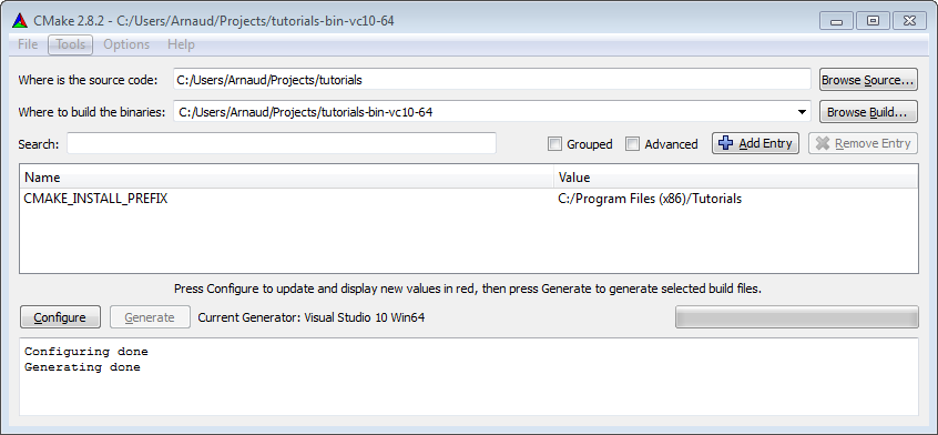
- Click on the Configure button. Since this is the first time you configure the project, CMake will ask you which compiler you would like to use. Choose wisely depending on step 1. If you have a 64 bit Windows, you can choose 64 bits; if you don’t know, choose 32 bits.
- Click on Configure until all red lines disappear. Click on Generate. Your Visual Studio project is now created. You can now forget about CMake.
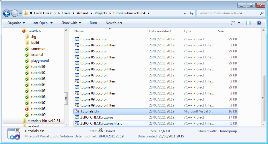
- Open C:\Users\XYZ\Projects\OpenGLTutorials-build-Visual2010-32bits. You will see a Tutorials.sln file : open it with Visual Studio.
In the Build menu, click Build All. Every tutorial and dependency will be compiled. Each executable will also be copied back into C:\Users\XYZ\Projects\OpenGLTutorials\ . Hopefuly no error occurs.
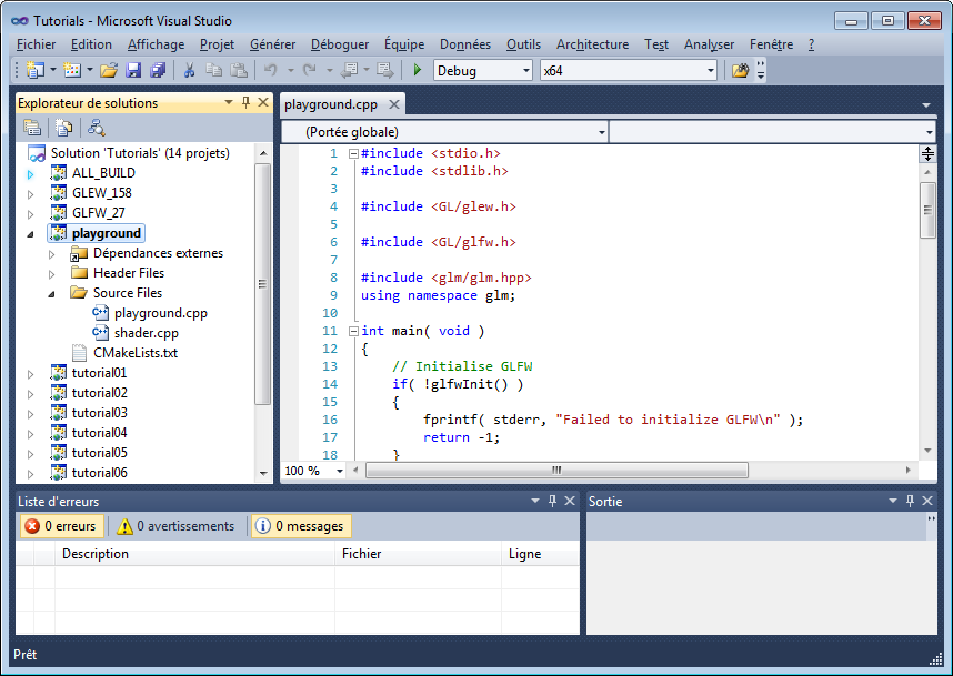
- Open C:\Users\XYZ\Projects\OpenGLTutorials\playground, and launch playground.exe. A black window should appear.
You can also launch any tutorial from inside Visual Studio. Right-click on Playground once, “Choose as startup project”. You can now debug the code by pressing F5.
Building on Linux
They are so many Linux variants out there that it’s impossible to list every possible platform. Adapt if required, and don’t hesitate to read your distribution’s documentation.
- Install the latest drivers. We highly recommend the closed-source binary drivers. It’s not GNU or whatever, but they work. If your distribution doesn’t provide an automatic install, try Ubuntu’s guide.
- Install all needed compilers, tools & libs. Complete list is : cmake make g++ libx11-dev libxi-dev libgl1-mesa-dev libglu1-mesa-dev libxrandr-dev libxext-dev libxcursor-dev libxinerama-dev libxi-dev . Use
sudo apt-get install *****orsu && yum install ******. - Download the source code and unzip it, for instance in ~/Projects/OpenGLTutorials/
-
cd in ~/Projects/OpenGLTutorials/ and enter the following commands :
- mkdir build
- cd build
-
cmake ..
- A makefile has been created in the build/ directory.
- type “make all”. Every tutorial and dependency will be compiled. Each executable will also be copied back into ~/Projects/OpenGLTutorials/ . Hopefuly no error occurs.
- Open ~/Projects/OpenGLTutorials/playground, and launch ./playground. A black window should appear.
Note that you really should use an IDE like Qt Creator. In particular, this one has built-in support for CMake, and it will provide a much nicer experience when debugging. Here are the instructions for QtCreator :
- In QtCreator, go to File->Tools->Options->Compile&Execute->CMake
- Set the path to CMake. This is most probably /usr/bin/cmake
- File->Open Project; Select tutorials/CMakeLists.txt
- Select a build directory, preferably outside the tutorials folder
- Optionally set -DCMAKE_BUILD_TYPE=Debug in the parameters box. Validate.
- Click on the hammer on the bottom. The tutorials can now be launched from the tutorials/ folder.
- To run the tutorials from QtCreator, click on Projects->Execution parameters->Working Directory, and select the directory where the shaders, textures & models live. Example for tutorial 2 : ~/opengl-tutorial/tutorial02_red_triangle/
Building on Mac
The procedure is very similar to Windows’ (Makefiles are also supported, but won’t be explained here) :
- Install XCode from the Mac App Store
- Download CMake, and install the .dmg . You don’t need to install the command-line tools.
- Download the source code and unzip it, for instance in ~/Projects/OpenGLTutorials/ .
- Launch CMake (Applications->CMake). In the first line, navigate to the unzipped folder. If unsure, choose the folder that contains the CMakeLists.txt file. In the second line, enter where you want all the compiler’s stuff to live. For instance, you can choose ~/Projects/OpenGLTutorials_bin_XCode/. Notice that it can be anywhere, not necessarily in the same folder.
- Click on the Configure button. Since this is the first time you configure the project, CMake will ask you which compiler you would like to use. Choose Xcode.
- Click on Configure until all red lines disappear. Click on Generate. Your Xcode project is now created. You can forget about CMake.
- Open ~/Projects/OpenGLTutorials_bin_XCode/ . You will see a Tutorials.xcodeproj file : open it.
- Select the desired tutorial to run in Xcode’s Scheme panel, and use the Run button to compile & run :
Note for Code::Blocks
Due to 2 bugs (one in C::B, one in CMake), you have to edit the command-line in Project->Build Options->Make commands, as follows :
You also have to setup the working directory yourself : Project->Properties -> Build targets -> tutorial N -> execution working dir ( it’s src_dir/tutorial_N/ ).
Running the tutorials
You should run the tutorials directly from the right directory : simply double-click on the executable. If you like command line best, cd to the right directory.
If you want to run the tutorials from the IDE, don’t forget to read the instructions above to set the correct working directory.
How to follow these tutorials
Each tutorial comes with its source code and data, which can be found in tutorialXX/. However, you will never modify these projects : they are for reference only. Open playground/playground.cpp, and tweak this file instead. Torture it in any way you like. If you are lost, simply cut’n paste any tutorial in it, and everything should be back to normal.
We will provide snippets of code all along the tutorials. Don’t hesitate to cut’n paste them directly in the playground while you’re reading : experimentation is good. Avoid simply reading the finished code, you won’t learn a lot this way. Even with simple cut’n pasting, you’ll get your boatload of problems.
Opening a window
Finally ! OpenGL code ! Well, not really. Many tutorials show you the “low level” way to do things, so that you can see that no magic happens. But the “open a window” part is actually very boring and useless, so we will use GLFW, an external library, to do this for us instead. If you really wanted to, you could use the Win32 API on Windows, the X11 API on Linux, and the Cocoa API on Mac; or use another high-level library like SFML, FreeGLUT, SDL, … see the Links page.
Ok, let’s go. First, we’ll have to deal with dependencies : we need some basic stuff to display messages in the console :
// Include standard headers
#include <stdio.h>
#include <stdlib.h>
First, GLEW. This one actually is a little bit magic, but let’s leave this for later.
// Include GLEW. Always include it before gl.h and glfw3.h, since it's a bit magic.
#include <GL/glew.h>
We decided to let GLFW handle the window and the keyboard, so let’s include it too :
// Include GLFW
#include <GLFW/glfw3.h>
We don’t actually need this one right now, but this is a library for 3D mathematics. It will prove very useful soon. There is no magic in GLM, you can write your own if you want; it’s just handy. The “using namespace” is there to avoid typing “glm::vec3”, but “vec3” instead.
// Include GLM
#include <glm/glm.hpp>
using namespace glm;
If you cut’n paste all these #include’s in playground.cpp, the compiler will complain that there is no main() function. So let’s create one :
int main(){
First thing to do it to initialize GLFW :
// Initialise GLFW
glewExperimental = true; // Needed for core profile
if( !glfwInit() )
{
    fprintf( stderr, "Failed to initialize GLFW\n" );
    return -1;
}
We can now create our first OpenGL window !
glfwWindowHint(GLFW_SAMPLES, 4); // 4x antialiasing
glfwWindowHint(GLFW_CONTEXT_VERSION_MAJOR, 3); // We want OpenGL 3.3
glfwWindowHint(GLFW_CONTEXT_VERSION_MINOR, 3);
glfwWindowHint(GLFW_OPENGL_FORWARD_COMPAT, GL_TRUE); // To make MacOS happy; should not be needed
glfwWindowHint(GLFW_OPENGL_PROFILE, GLFW_OPENGL_CORE_PROFILE); // We don't want the old OpenGL

// Open a window and create its OpenGL context
GLFWwindow* window; // (In the accompanying source code, this variable is global for simplicity)
window = glfwCreateWindow( 1024, 768, "Tutorial 01", NULL, NULL);
if( window == NULL ){
    fprintf( stderr, "Failed to open GLFW window. If you have an Intel GPU, they are not 3.3 compatible. Try the 2.1 version of the tutorials.\n" );
    glfwTerminate();
    return -1;
}
glfwMakeContextCurrent(window); // Initialize GLEW
glewExperimental=true; // Needed in core profile
if (glewInit() != GLEW_OK) {
    fprintf(stderr, "Failed to initialize GLEW\n");
    return -1;
}
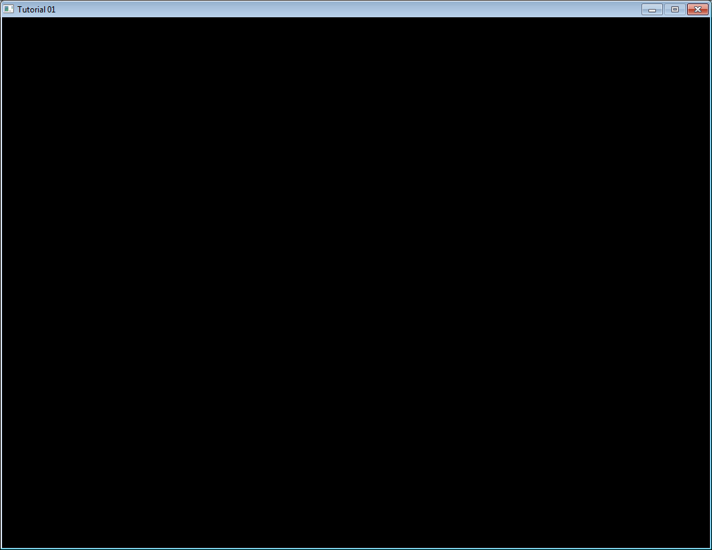
Build this and run. A window should appear, and be closed right away. Of course! We need to wait until the user hits the Escape key :
// Ensure we can capture the escape key being pressed below
glfwSetInputMode(window, GLFW_STICKY_KEYS, GL_TRUE);

do{
    // Clear the screen. It's not mentioned before Tutorial 02, but it can cause flickering, so it's there nonetheless.
    glClear( GL_COLOR_BUFFER_BIT );

    // Draw nothing, see you in tutorial 2 !

    // Swap buffers
    glfwSwapBuffers(window);
    glfwPollEvents();

} // Check if the ESC key was pressed or the window was closed
while( glfwGetKey(window, GLFW_KEY_ESCAPE ) != GLFW_PRESS &&
       glfwWindowShouldClose(window) == 0 );
And this concludes our first tutorial ! In Tutorial 2, you will learn how to actually draw a triangle.
Tutorial 2 : The first triangle
This will be another long tutorial.
OpenGL 3 makes it easy to write complicated stuff, but at the expense that drawing a simple triangle is actually quite difficult.
Don’t forget to cut’n paste the code on a regular basis.
If the program crashes at startup, you’re probably running from the wrong directory. Read CAREFULLY the first tutorial and the FAQ on how to configure Visual Studio !
The VAO
I won’t dig into details now, but you need to create a Vertex Array Object and set it as the current one :
GLuint VertexArrayID;
glGenVertexArrays(1, &VertexArrayID);
glBindVertexArray(VertexArrayID);
Do this once your window is created (= after the OpenGL Context creation) and before any other OpenGL call.
If you really want to know more about VAOs, there are a few other tutorials out there, but this is not very important.
Screen Coordinates
A triangle is defined by three points. When talking about “points” in 3D graphics, we usually use the word “vertex” ( “vertices” on the plural ). A vertex has 3 coordinates : X, Y and Z. You can think about these three coordinates in the following way :
- X in on your right
- Y is up
- Z is towards your back (yes, behind, not in front of you)
But here is a better way to visualize this : use the Right Hand Rule
- X is your thumb
- Y is your index
- Z is your middle finger. If you put your thumb to the right and your index to the sky, it will point to your back, too.
Having the Z in this direction is weird, so why is it so ? Short answer : because 100 years of Right Hand Rule Math will give you lots of useful tools. The only downside is an unintuitive Z.
On a side note, notice that you can move your hand freely : your X, Y and Z will be moving, too. More on this later.
So we need three 3D points in order to make a triangle ; let’s go :
// An array of 3 vectors which represents 3 vertices
static const GLfloat g_vertex_buffer_data[] = {
   -1.0f, -1.0f, 0.0f,
   1.0f, -1.0f, 0.0f,
   0.0f,  1.0f, 0.0f,
};
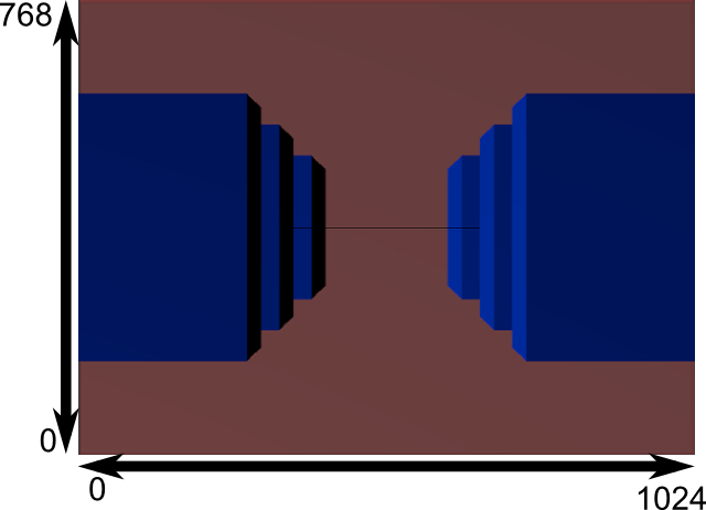
The first vertex is (-1,-1,0). This means that unless we transform it in some way, it will be displayed at (-1,-1) on the screen. What does this mean ? The screen origin is in the middle, X is on the right, as usual, and Y is up. This is what it gives on a wide screen :
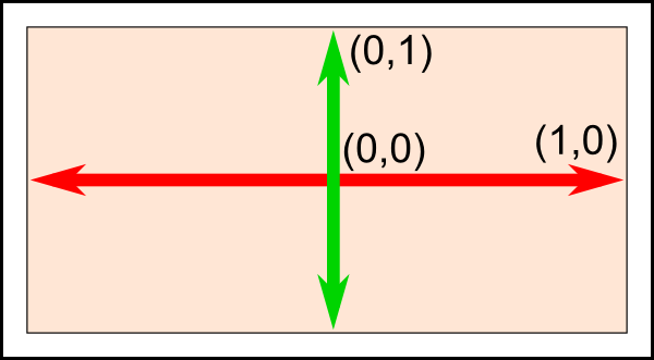
This is something you can’t change, it’s built in your graphics card. So (-1,-1) is the bottom left corner of your screen. (1,-1) is the bottom right, and (0,1) is the middle top. So this triangle should take most of the screen.
Drawing our triangle
The next step is to give this triangle to OpenGL. We do this by creating a buffer:
// This will identify our vertex buffer
GLuint vertexbuffer;
// Generate 1 buffer, put the resulting identifier in vertexbuffer
glGenBuffers(1, &vertexbuffer);
// The following commands will talk about our 'vertexbuffer' buffer
glBindBuffer(GL_ARRAY_BUFFER, vertexbuffer);
// Give our vertices to OpenGL.
glBufferData(GL_ARRAY_BUFFER, sizeof(g_vertex_buffer_data), g_vertex_buffer_data, GL_STATIC_DRAW);
This needs to be done only once.
Now, in our main loop, where we used to draw “nothing”, we can draw our magnificent triangle :
// 1st attribute buffer : vertices
glEnableVertexAttribArray(0);
glBindBuffer(GL_ARRAY_BUFFER, vertexbuffer);
glVertexAttribPointer(
   0,                  // attribute 0. No particular reason for 0, but must match the layout in the shader.
   3,                  // size
   GL_FLOAT,           // type
   GL_FALSE,           // normalized?
   0,                  // stride
   (void*)0            // array buffer offset
);
// Draw the triangle !
glDrawArrays(GL_TRIANGLES, 0, 3); // Starting from vertex 0; 3 vertices total -> 1 triangle
glDisableVertexAttribArray(0);
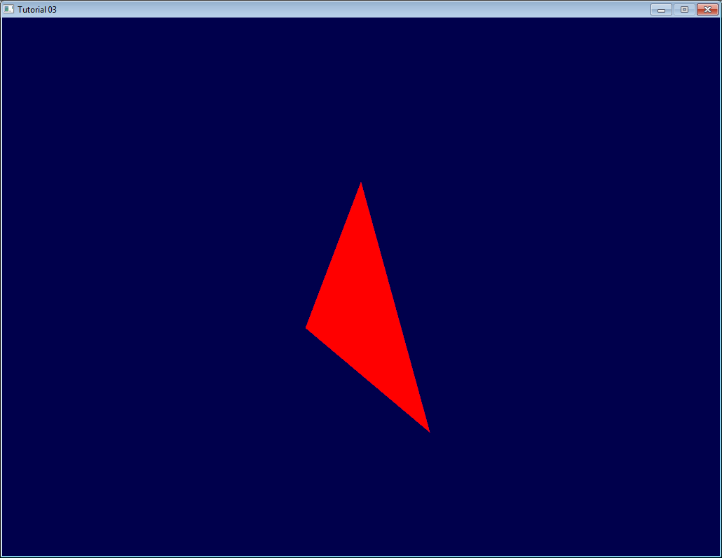
If you’re lucky, you can see the result in white. (Don’t panic if you don’t some systems require a shader to show anything) :
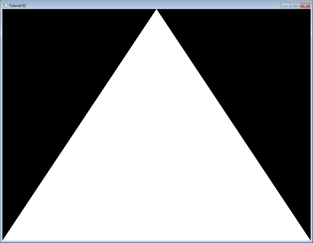
Now this is some boring white. Let’s see how we can improve it by painting it in red. This is done by using something called shaders.
Shaders
Shader Compilation
In the simplest possible configuration, you will need two shaders : one called Vertex Shader, which will be executed for each vertex, and one called Fragment Shader, which will be executed for each sample. And since we use 4x antialising, we have 4 samples in each pixel.
Shaders are programmed in a language called GLSL : GL Shader Language, which is part of OpenGL. Unlike C or Java, GLSL has to be compiled at run time, which means that each and every time you launch your application, all your shaders are recompiled.
The two shaders are usually in separate files. In this example, we have SimpleFragmentShader.fragmentshader and SimpleVertexShader.vertexshader . The extension is irrelevant, it could be .txt or .glsl .
So here’s the code. It’s not very important to fully understand it, since you often do this only once in a program, so comments should be enough. Since this function will be used by all other tutorials, it is placed in a separate file : common/loadShader.cpp . Notice that just as buffers, shaders are not directly accessible : we just have an ID. The actual implementation is hidden inside the driver.
GLuint LoadShaders(const char * vertex_file_path,const char * fragment_file_path){

	// Create the shaders
	GLuint VertexShaderID = glCreateShader(GL_VERTEX_SHADER);
	GLuint FragmentShaderID = glCreateShader(GL_FRAGMENT_SHADER);

	// Read the Vertex Shader code from the file
	std::string VertexShaderCode;
	std::ifstream VertexShaderStream(vertex_file_path, std::ios::in);
	if(VertexShaderStream.is_open()){
		std::stringstream sstr;
		sstr << VertexShaderStream.rdbuf();
		VertexShaderCode = sstr.str();
		VertexShaderStream.close();
	}else{
		printf("Impossible to open %s. Are you in the right directory ? Don't forget to read the FAQ !\n", vertex_file_path);
		getchar();
		return 0;
	}

	// Read the Fragment Shader code from the file
	std::string FragmentShaderCode;
	std::ifstream FragmentShaderStream(fragment_file_path, std::ios::in);
	if(FragmentShaderStream.is_open()){
		std::stringstream sstr;
		sstr << FragmentShaderStream.rdbuf();
		FragmentShaderCode = sstr.str();
		FragmentShaderStream.close();
	}

	GLint Result = GL_FALSE;
	int InfoLogLength;

	// Compile Vertex Shader
	printf("Compiling shader : %s\n", vertex_file_path);
	char const * VertexSourcePointer = VertexShaderCode.c_str();
	glShaderSource(VertexShaderID, 1, &VertexSourcePointer , NULL);
	glCompileShader(VertexShaderID);

	// Check Vertex Shader
	glGetShaderiv(VertexShaderID, GL_COMPILE_STATUS, &Result);
	glGetShaderiv(VertexShaderID, GL_INFO_LOG_LENGTH, &InfoLogLength);
	if ( InfoLogLength > 0 ){
		std::vector<char> VertexShaderErrorMessage(InfoLogLength+1);
		glGetShaderInfoLog(VertexShaderID, InfoLogLength, NULL, &VertexShaderErrorMessage[0]);
		printf("%s\n", &VertexShaderErrorMessage[0]);
	}

	// Compile Fragment Shader
	printf("Compiling shader : %s\n", fragment_file_path);
	char const * FragmentSourcePointer = FragmentShaderCode.c_str();
	glShaderSource(FragmentShaderID, 1, &FragmentSourcePointer , NULL);
	glCompileShader(FragmentShaderID);

	// Check Fragment Shader
	glGetShaderiv(FragmentShaderID, GL_COMPILE_STATUS, &Result);
	glGetShaderiv(FragmentShaderID, GL_INFO_LOG_LENGTH, &InfoLogLength);
	if ( InfoLogLength > 0 ){
		std::vector<char> FragmentShaderErrorMessage(InfoLogLength+1);
		glGetShaderInfoLog(FragmentShaderID, InfoLogLength, NULL, &FragmentShaderErrorMessage[0]);
		printf("%s\n", &FragmentShaderErrorMessage[0]);
	}

	// Link the program
	printf("Linking program\n");
	GLuint ProgramID = glCreateProgram();
	glAttachShader(ProgramID, VertexShaderID);
	glAttachShader(ProgramID, FragmentShaderID);
	glLinkProgram(ProgramID);

	// Check the program
	glGetProgramiv(ProgramID, GL_LINK_STATUS, &Result);
	glGetProgramiv(ProgramID, GL_INFO_LOG_LENGTH, &InfoLogLength);
	if ( InfoLogLength > 0 ){
		std::vector<char> ProgramErrorMessage(InfoLogLength+1);
		glGetProgramInfoLog(ProgramID, InfoLogLength, NULL, &ProgramErrorMessage[0]);
		printf("%s\n", &ProgramErrorMessage[0]);
	}

	glDetachShader(ProgramID, VertexShaderID);
	glDetachShader(ProgramID, FragmentShaderID);

	glDeleteShader(VertexShaderID);
	glDeleteShader(FragmentShaderID);

	return ProgramID;
}
Our Vertex Shader
Let’s write our vertex shader first. The first line tells the compiler that we will use OpenGL 3’s syntax.
#version 330 core
The second line declares the input data :
layout(location = 0) in vec3 vertexPosition_modelspace;
Let’s explain this line in detail :
- “vec3” is a vector of 3 components in GLSL. It is similar (but different) to the glm::vec3 we used to declare our triangle. The important thing is that if we use 3 components in C++, we use 3 components in GLSL too.
- “layout(location = 0)” refers to the buffer we use to feed the vertexPosition_modelspace attribute. Each vertex can have numerous attributes : A position, one or several colours, one or several texture coordinates, lots of other things. OpenGL doesn’t know what a colour is : it just sees a vec3. So we have to tell him which buffer corresponds to which input. We do that by setting the layout to the same value as the first parameter to glVertexAttribPointer. The value “0” is not important, it could be 12 (but no more than glGetIntegerv(GL_MAX_VERTEX_ATTRIBS, &v) ), the important thing is that it’s the same number on both sides.
- “vertexPosition_modelspace” could have any other name. It will contain the position of the vertex for each run of the vertex shader.
- “in” means that this is some input data. Soon we’ll see the “out” keyword.
The function that is called for each vertex is called main, just as in C :
void main(){
Our main function will merely set the vertex’ position to whatever was in the buffer. So if we gave (1,1), the triangle would have one of its vertices at the top right corner of the screen. We’ll see in the next tutorial how to do some more interesting computations on the input position.
  gl_Position.xyz = vertexPosition_modelspace;
  gl_Position.w = 1.0;
}
gl_Position is one of the few built-in variables : you *have *to assign some value to it. Everything else is optional; we’ll see what “everything else” means in Tutorial 4.
Our Fragment Shader
For our first fragment shader, we will do something really simple : set the color of each fragment to red. (Remember, there are 4 fragment in a pixel because we use 4x AA)
#version 330 core
out vec3 color;
void main(){
  color = vec3(1,0,0);
}
So yeah, vec3(1,0,0) means red. This is because on computer screens, colour is represented by a Red, Green, and Blue triplet, in this order. So (1,0,0) means Full Red, no green and no blue.
Putting it all together
Import our LoadShaders function as the last include:
#include <common/shader.hpp>
Before the main loop, call our LoadShaders function:
// Create and compile our GLSL program from the shaders
GLuint programID = LoadShaders( "SimpleVertexShader.vertexshader", "SimpleFragmentShader.fragmentshader" );
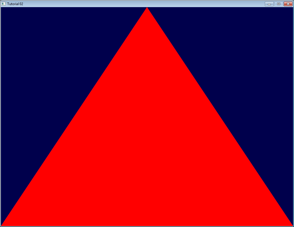
Now inside the main loop, first clear the screen. This will change the background color to dark blue because of the previous glClearColor(0.0f, 0.0f, 0.4f, 0.0f) call:
glClear(GL_COLOR_BUFFER_BIT | GL_DEPTH_BUFFER_BIT);
and then tell OpenGL that you want to use your shader:
// Use our shader
glUseProgram(programID);
// Draw triangle...
… and presto, here’s your red triangle !
In the next tutorial we’ll learn transformations : How to setup your camera, move your objects, etc.
Tutorial 3: Matrices
- Homogeneous coordinates
- Transformation matrices
- The Model, View and Projection matrices
- Putting it all together
- Exercises
The engines don’t move the ship at all. The ship stays where it is and the engines move the universe around it.
Futurama
This is the single most important tutorial of the whole set. Be sure to read it at least eight times.
Homogeneous coordinates
Until then, we only considered 3D vertices as a (x,y,z) triplet. Let’s introduce w. We will now have (x,y,z,w) vectors.
This will be more clear soon, but for now, just remember this:
- If w == 1, then the vector (x,y,z,1) is a position in space.
- If w == 0, then the vector (x,y,z,0) is a direction.
(In fact, remember this forever.)
What difference does this make? Well, for a rotation, it doesn’t change anything. When you rotate a point or a direction, you get the same result. However, for a translation (when you move the point in a certain direction), things are different. What could mean “translate a direction”? Not much.
Homogeneous coordinates allow us to use a single mathematical formula to deal with these two cases.
Transformation matrices
An introduction to matrices
Simply put, a matrix is an array of numbers with a predefined number of rows and colums. For instance, a 2x3 matrix can look like this:

In 3D graphics we will mostly use 4x4 matrices. They will allow us to transform our (x,y,z,w) vertices. This is done by multiplying the vertex with the matrix:
Matrix x Vertex (in this order!!) = TransformedVertex

This isn’t as scary as it looks. Put your left finger on the a, and your right finger on the x. This is ax. Move your left finger to the next number (b), and your right finger to the next number (y). You’ve got by. Once again: cz. Once again: dw. ax + by + cz + dw. You’ve got your new x! Do the same for each line, and you’ll get your new (x,y,z,w) vector.
Now this is quite boring to compute, and we will do this often, so let’s ask the computer to do it instead.
In C++, with GLM:
glm::mat4 myMatrix;
glm::vec4 myVector;
// fill myMatrix and myVector somehow
glm::vec4 transformedVector = myMatrix * myVector; // Again, in this order! This is important.
In GLSL:
mat4 myMatrix;
vec4 myVector;
// fill myMatrix and myVector somehow
vec4 transformedVector = myMatrix * myVector; // Yeah, it's pretty much the same as GLM
(have you cut ‘n’ pasted this in your code? Go on, try it!)
Translation matrices
These are the most simple tranformation matrices to understand. A translation matrix look like this:
![]()
where X,Y,Z are the values that you want to add to your position.
So if we want to translate the vector (10,10,10,1) of 10 units in the X direction, we get:
![]()
(do it! doooooo it)
…and we get a (20,10,10,1) homogeneous vector! Remember, the 1 means that it is a position, not a direction. So our transformation didn’t change the fact that we were dealing with a position, which is good.
Let’s now see what happens to a vector that represents a direction towards the -z axis: (0,0,-1,0)
![]()
…i.e. our original (0,0,-1,0) direction, which is great because, as I said ealier, moving a direction does not make sense.
So, how does this translate to code?
In C++, with GLM:
#include <glm/gtx/transform.hpp> // after <glm/glm.hpp>

glm::mat4 myMatrix = glm::translate(glm::mat4(), glm::vec3(10.0f, 0.0f, 0.0f));
glm::vec4 myVector(10.0f, 10.0f, 10.0f, 0.0f);
glm::vec4 transformedVector = myMatrix * myVector; // guess the result
In GLSL:
vec4 transformedVector = myMatrix * myVector;
Well, in fact, you almost never do this in GLSL. Most of the time, you use glm::translate() in C++ to compute your matrix, send it to GLSL, and do only the multiplication:
The Identity matrix
This one is special. It doesn’t do anything. But I mention it because it’s as important as knowing that multiplying A by 1.0 gives A.
In C++:
glm::mat4 myIdentityMatrix = glm::mat4(1.0f);
Scaling matrices
Scaling matrices are quite easy too:

So if you want to scale a vector (position or direction, it doesn’t matter) by 2.0 in all directions:
and the w still didn’t change. You may ask: what is the meaning of “scaling a direction”? Well, often, not much, so you usually don’t do such a thing, but in some (rare) cases it can be handy.
(notice that the identity matrix is only a special case of scaling matrices, with (X,Y,Z) = (1,1,1). It’s also a special case of translation matrix with (X,Y,Z)=(0,0,0), by the way)
In C++:
// Use #include <glm/gtc/matrix_transform.hpp> and #include <glm/gtx/transform.hpp>
glm::mat4 myScalingMatrix = glm::scale(glm::mat4(1), glm::vec3(2,2,2));
Rotation matrices
These are quite complicated. I’ll skip the details here, as it’s not important to know their exact layout for everyday use. For more information, please have a look to the Matrices and Quaternions FAQ (popular resource, probably available in your language as well). You can also have a look at the Rotations tutorials.
In C++:
// Use #include <glm/gtc/matrix_transform.hpp> and #include <glm/gtx/transform.hpp>
glm::vec3 myRotationAxis(??,??,??);
glm::rotate( angle_in_degrees, myRotationAxis );
Cumulating transformations
So now we know how to rotate, translate, and scale our vectors. It would be great to combine these transformations. This is done by multiplying the matrices together, for instance:
TransformedVector = TranslationMatrix * RotationMatrix * ScaleMatrix * OriginalVector;
!!! BEWARE!!! This lines actually performs the scaling FIRST, and THEN the rotation, and THEN the translation. This is how matrix multiplication works.
Writing the operations in another order wouldn’t produce the same result. Try it yourself:
-
make one step ahead (beware of your computer) and turn left;
-
turn left, and make one step ahead
As a matter of fact, the order above is what you will usually need for game characters and other items: Scale it first if needed; then set its direction, then translate it. For instance, given a ship model (rotations have been removed for simplification):
- The wrong way:
- You translate the ship by (10,0,0). Its center is now at 10 units of the origin.
- You scale your ship by 2. Every coordinate is multiplied by 2 relative to the origin, which is far away… So you end up with a big ship, but centered at 2*10 = 20. Which you don’t want.
- The right way:
- You scale your ship by 2. You get a big ship, centered on the origin.
- You translate your ship. It’s still the same size, and at the right distance.
Matrix-matrix multiplication is very similar to matrix-vector multiplication, so I’ll once again skip some details and redirect you the the Matrices and Quaternions FAQ if needed. For now, we’ll simply ask the computer to do it:
in C++, with GLM:
glm::mat4 myModelMatrix = myTranslationMatrix * myRotationMatrix * myScaleMatrix;
glm::vec4 myTransformedVector = myModelMatrix * myOriginalVector;
in GLSL:
mat4 transform = mat2 * mat1;
vec4 out_vec = transform * in_vec;
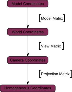
The Model, View and Projection matrices
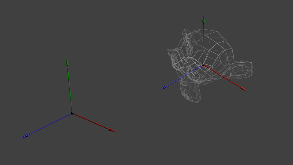
For the rest of this tutorial, we will suppose that we know how to draw Blender’s favourite 3d model: the monkey Suzanne.
The Model, View and Projection matrices are a handy tool to separate transformations cleanly. You may not use this (after all, that’s what we did in tutorials 1 and 2). But you should. This is the way everybody does, because it’s easier this way.
The Model matrix
This model, just as our beloved red triangle, is defined by a set of vertices. The X,Y,Z coordinates of these vertices are defined relative to the object’s center: that is, if a vertex is at (0,0,0), it is at the center of the object.
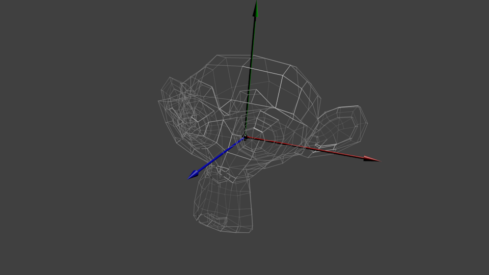
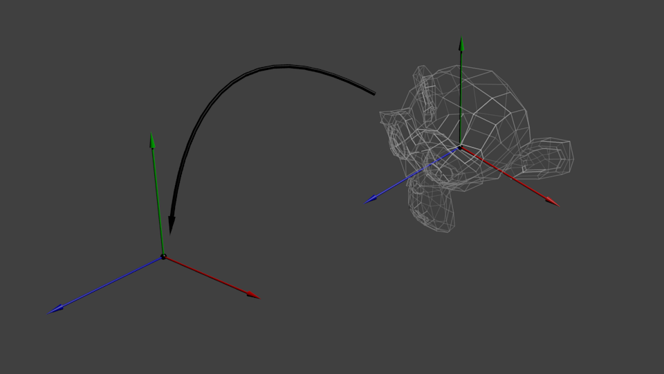
We’d like to be able to move this model, maybe because the player controls it with the keyboard and the mouse. Easy, you just learnt do do so: translation\*rotation\*scale, and done. You apply this matrix to all your vertices at each frame (in GLSL, not in C++!) and everything moves. Something that doesn’t move will be at the center of the world.
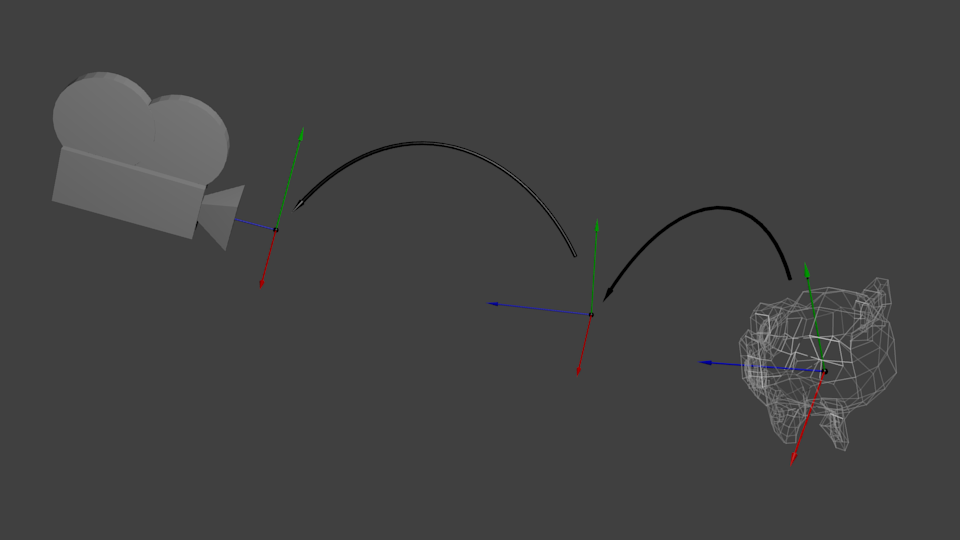
Your vertices are now in World Space. This is the meaning of the black arrow in the image below: We went from Model Space (all vertices defined relatively to the center of the model) to World Space (all vertices defined relatively to the center of the world).
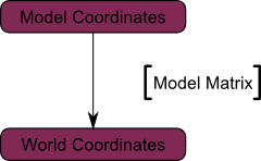
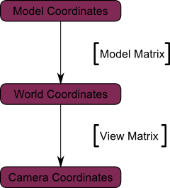
We can sum this up with the following diagram:
The View matrix
Let’s quote Futurama again:
The engines don’t move the ship at all. The ship stays where it is and the engines move the universe around it.
When you think about it, the same applies to cameras. It you want to view a moutain from another angle, you can either move the camera…or move the mountain. While not practical in real life, this is really simple and handy in Computer Graphics.
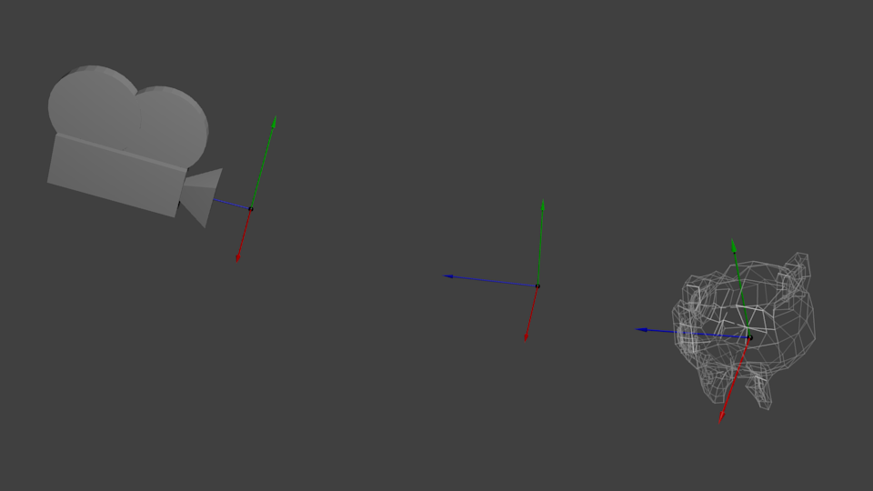
So initially your camera is at the origin of the World Space. In order to move the world, you simply introduce another matrix. Let’s say you want to move your camera of 3 units to the right (+X). This is equivalent to moving your whole world (meshes included) 3 units to the LEFT! (-X). While you brain melts, let’s do it:
// Use #include <glm/gtc/matrix_transform.hpp> and #include <glm/gtx/transform.hpp>
glm::mat4 ViewMatrix = glm::translate(glm::mat4(), glm::vec3(-3.0f, 0.0f ,0.0f));
Again, the image below illustrates this: We went from World Space (all vertices defined relatively to the center of the world, as we made so in the previous section) to Camera Space (all vertices defined relatively to the camera).
Before you head explodes from this, enjoy GLM’s great glm::lookAt function:
glm::mat4 CameraMatrix = glm::lookAt(
    cameraPosition, // the position of your camera, in world space
    cameraTarget,   // where you want to look at, in world space
    upVector        // probably glm::vec3(0,1,0), but (0,-1,0) would make you looking upside-down, which can be great too
);
Here’s the compulsory diagram:
This is not over yet, though.
The Projection matrix
We’re now in Camera Space. This means that after all theses transformations, a vertex that happens to have x==0 and y==0 should be rendered at the center of the screen. But we can’t use only the x and y coordinates to determine where an object should be put on the screen: its distance to the camera (z) counts, too! For two vertices with similar x and y coordinates, the vertex with the biggest z coordinate will be more on the center of the screen than the other.
This is called a perspective projection:
And luckily for us, a 4x4 matrix can represent this projection1:
// Generates a really hard-to-read matrix, but a normal, standard 4x4 matrix nonetheless
glm::mat4 projectionMatrix = glm::perspective(
    glm::radians(FoV), // The vertical Field of View, in radians: the amount of "zoom". Think "camera lens". Usually between 90° (extra wide) and 30° (quite zoomed in)
    4.0f / 3.0f,       // Aspect Ratio. Depends on the size of your window. Notice that 4/3 == 800/600 == 1280/960, sounds familiar?
    0.1f,              // Near clipping plane. Keep as big as possible, or you'll get precision issues.
    100.0f             // Far clipping plane. Keep as little as possible.
);
One last time:
We went from Camera Space (all vertices defined relatively to the camera) to Homogeneous Space (all vertices defined in a small cube. Everything inside the cube is onscreen).
And the final diagram:
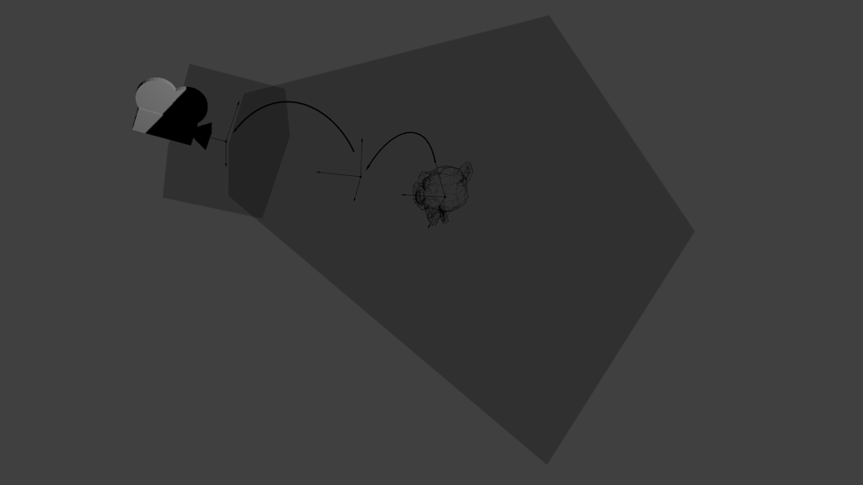
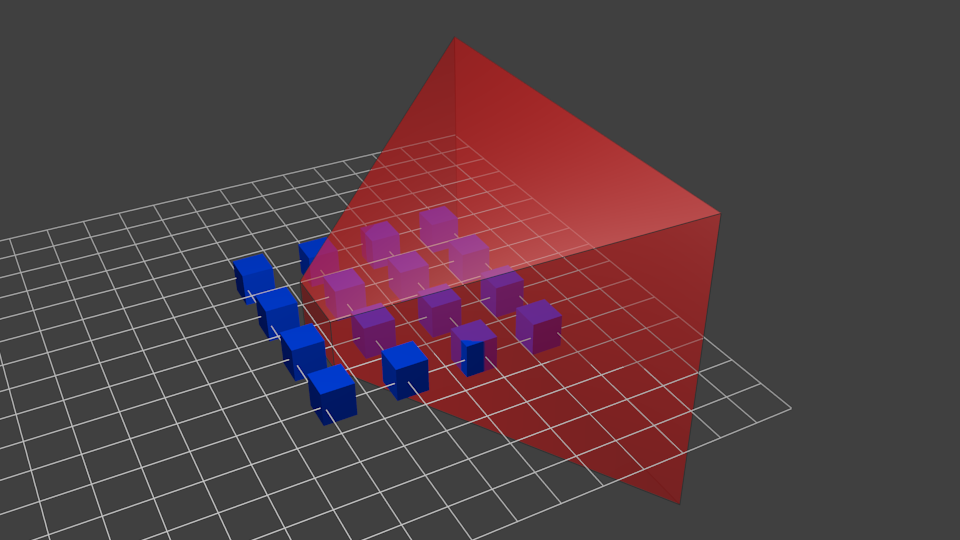
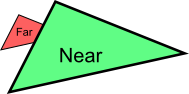
Here’s another diagram so that you understand better what happens with this Projection stuff. Before projection, we’ve got our blue objects, in Camera Space, and the red shape represents the frustum of the camera: the part of the scene that the camera is actually able to see.
Multiplying everything by the Projection Matrix has the following effect:
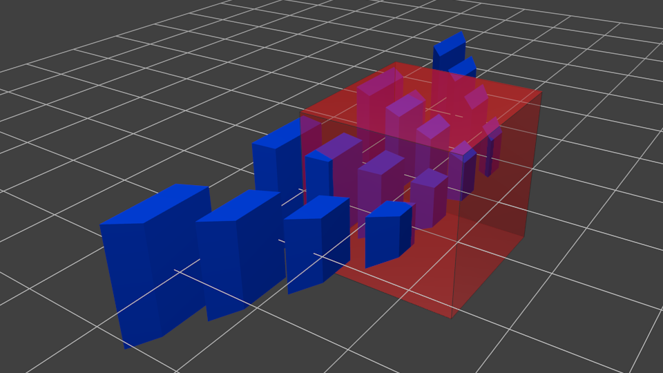
In this image, the frustum is now a perfect cube (between -1 and 1 on all axes, it’s a little bit hard to see it), and all blue objects have been deformed in the same way. Thus, the objects that are near the camera ( = near the face of the cube that we can’t see) are big, the others are smaller. Seems like real life!
Let’s see what it looks like from the “behind” the frustum:
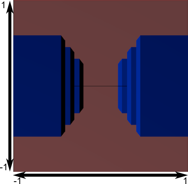
Here you get your image! It’s just a little bit too square, so another mathematical transformation is applied (this one is automatic, you don’t have to do it yourself in the shader) to fit this to the actual window size:
And this is the image that is actually rendered!
Cumulating transformations: the ModelViewProjection matrix
…Just a standard matrix multiplication as you already love them!
// C++: compute the matrix
glm::mat4 MVPmatrix = projection * view * model; // Remember: inverted!
// GLSL: apply it
transformed_vertex = MVP * in_vertex;
Putting it all together
- First step: include the GLM GTC matrix transform functions:
#include <glm/gtc/matrix_transform.hpp>
-
Second step: generating our MVP matrix. This must be done for each model you render.
// Projection matrix: 45° Field of View, 4:3 ratio, display range: 0.1 unit <-> 100 units glm::mat4 Projection = glm::perspective(glm::radians(45.0f), (float) width / (float)height, 0.1f, 100.0f); // Or, for an ortho camera: //glm::mat4 Projection = glm::ortho(-10.0f,10.0f,-10.0f,10.0f,0.0f,100.0f); // In world coordinates // Camera matrix glm::mat4 View = glm::lookAt( glm::vec3(4,3,3), // Camera is at (4,3,3), in World Space glm::vec3(0,0,0), // and looks at the origin glm::vec3(0,1,0) // Head is up (set to 0,-1,0 to look upside-down) ); // Model matrix: an identity matrix (model will be at the origin) glm::mat4 Model = glm::mat4(1.0f); // Our ModelViewProjection: multiplication of our 3 matrices glm::mat4 mvp = Projection * View * Model; // Remember, matrix multiplication is the other way around -
Third step: give it to GLSL
// Get a handle for our "MVP" uniform // Only during the initialisation GLuint MatrixID = glGetUniformLocation(programID, "MVP"); // Send our transformation to the currently bound shader, in the "MVP" uniform // This is done in the main loop since each model will have a different MVP matrix (At least for the M part) glUniformMatrix4fv(MatrixID, 1, GL_FALSE, &mvp[0][0]); -
Fourth step: use it in GLSL to transform our vertices in
SimpleVertexShader.vertexshader// Input vertex data, different for all executions of this shader. layout(location = 0) in vec3 vertexPosition_modelspace; // Values that stay constant for the whole mesh. uniform mat4 MVP; void main(){ // Output position of the vertex, in clip space: MVP * position gl_Position = MVP * vec4(vertexPosition_modelspace,1); } -
Done! Here is the same triangle as in tutorial 2, still at the origin (0,0,0), but viewed in perspective from point (4,3,3), heads up (0,1,0), with a 45° field of view.
In tutorial 6 you’ll learn how to modify these values dynamically using the keyboard and the mouse to create a game-like camera, but first, we’ll learn how to give our 3D models some colour (tutorial 4) and textures (tutorial 5).
Exercises
- Try changing the glm::perspective
- Instead of using a perspective projection, use an orthographic projection (glm::ortho)
- Modify ModelMatrix to translate, rotate, then scale the triangle
- Do the same thing, but in different orders. What do you notice? What is the “best” order that you would want to use for a character?
Addendum
-
[…]luckily for us, a 4x4 matrix can represent this projection: Actually, this is not correct. A perspective transformation is not affine, and as such, can’t be represented entirely by a matrix. After beeing multiplied by the ProjectionMatrix, homogeneous coordinates are divided by their own W component. This W component happens to be -Z (because the projection matrix has been crafted this way). This way, points that are far away from the origin are divided by a big Z; their X and Y coordinates become smaller; points become more close to each other, objects seem smaller; and this is what gives the perspective. This transformation is done in hardware, and is not visible in the shader. ↩
Tutorial 4 : A Colored Cube
Welcome for the 4rth tutorial ! You will do the following :
- Draw a cube instead of the boring triangle
- Add some fancy colors
- Learn what the Z-Buffer is
Draw a cube
A cube has six square faces. Since OpenGL only knows about triangles, we’ll have to draw 12 triangles : two for each face. We just define our vertices in the same way as we did for the triangle.
// Our vertices. Three consecutive floats give a 3D vertex; Three consecutive vertices give a triangle.
// A cube has 6 faces with 2 triangles each, so this makes 6*2=12 triangles, and 12*3 vertices
static const GLfloat g_vertex_buffer_data[] = {
    -1.0f,-1.0f,-1.0f, // triangle 1 : begin
    -1.0f,-1.0f, 1.0f,
    -1.0f, 1.0f, 1.0f, // triangle 1 : end
    1.0f, 1.0f,-1.0f, // triangle 2 : begin
    -1.0f,-1.0f,-1.0f,
    -1.0f, 1.0f,-1.0f, // triangle 2 : end
    1.0f,-1.0f, 1.0f,
    -1.0f,-1.0f,-1.0f,
    1.0f,-1.0f,-1.0f,
    1.0f, 1.0f,-1.0f,
    1.0f,-1.0f,-1.0f,
    -1.0f,-1.0f,-1.0f,
    -1.0f,-1.0f,-1.0f,
    -1.0f, 1.0f, 1.0f,
    -1.0f, 1.0f,-1.0f,
    1.0f,-1.0f, 1.0f,
    -1.0f,-1.0f, 1.0f,
    -1.0f,-1.0f,-1.0f,
    -1.0f, 1.0f, 1.0f,
    -1.0f,-1.0f, 1.0f,
    1.0f,-1.0f, 1.0f,
    1.0f, 1.0f, 1.0f,
    1.0f,-1.0f,-1.0f,
    1.0f, 1.0f,-1.0f,
    1.0f,-1.0f,-1.0f,
    1.0f, 1.0f, 1.0f,
    1.0f,-1.0f, 1.0f,
    1.0f, 1.0f, 1.0f,
    1.0f, 1.0f,-1.0f,
    -1.0f, 1.0f,-1.0f,
    1.0f, 1.0f, 1.0f,
    -1.0f, 1.0f,-1.0f,
    -1.0f, 1.0f, 1.0f,
    1.0f, 1.0f, 1.0f,
    -1.0f, 1.0f, 1.0f,
    1.0f,-1.0f, 1.0f
};
The OpenGL buffer is created, bound, filled and configured with the standard functions (glGenBuffers, glBindBuffer, glBufferData, glVertexAttribPointer) ; see Tutorial 2 for a quick reminder. The draw call does not change either, you just have to set the right number of vertices that must be drawn :
// Draw the triangle !
glDrawArrays(GL_TRIANGLES, 0, 12*3); // 12*3 indices starting at 0 -> 12 triangles -> 6 squares
A few remarks on this code :
- For now, our 3D model is fixed : in order to change it, you have to modify the source code, recompile the application, and hope for the best. We’ll learn how to load dynamic models in tutorial 7.
- Each vertex is actually written at least 3 times (search “-1.0f,-1.0f,-1.0f” in the code above). This is an awful waste of memory. We’ll learn how to deal with this in tutorial 9.
You now have all the needed pieces to draw the cube in white. Make the shaders work ! go on, at least try :)
Adding colors
A color is, conceptually, exactly the same as a position : it’s just data. In OpenGL terms, they are “attributes”. As a matter of fact, we already used this with glEnableVertexAttribArray() and glVertexAttribPointer(). Let’s add another attribute. The code is going to be very similar.
First, declare your colors : one RGB triplet per vertex. Here I generated some randomly, so the result won’t look that good, but you can do something better, for instance by copying the vertex’s position into its own color.
// One color for each vertex. They were generated randomly.
static const GLfloat g_color_buffer_data[] = {
    0.583f,  0.771f,  0.014f,
    0.609f,  0.115f,  0.436f,
    0.327f,  0.483f,  0.844f,
    0.822f,  0.569f,  0.201f,
    0.435f,  0.602f,  0.223f,
    0.310f,  0.747f,  0.185f,
    0.597f,  0.770f,  0.761f,
    0.559f,  0.436f,  0.730f,
    0.359f,  0.583f,  0.152f,
    0.483f,  0.596f,  0.789f,
    0.559f,  0.861f,  0.639f,
    0.195f,  0.548f,  0.859f,
    0.014f,  0.184f,  0.576f,
    0.771f,  0.328f,  0.970f,
    0.406f,  0.615f,  0.116f,
    0.676f,  0.977f,  0.133f,
    0.971f,  0.572f,  0.833f,
    0.140f,  0.616f,  0.489f,
    0.997f,  0.513f,  0.064f,
    0.945f,  0.719f,  0.592f,
    0.543f,  0.021f,  0.978f,
    0.279f,  0.317f,  0.505f,
    0.167f,  0.620f,  0.077f,
    0.347f,  0.857f,  0.137f,
    0.055f,  0.953f,  0.042f,
    0.714f,  0.505f,  0.345f,
    0.783f,  0.290f,  0.734f,
    0.722f,  0.645f,  0.174f,
    0.302f,  0.455f,  0.848f,
    0.225f,  0.587f,  0.040f,
    0.517f,  0.713f,  0.338f,
    0.053f,  0.959f,  0.120f,
    0.393f,  0.621f,  0.362f,
    0.673f,  0.211f,  0.457f,
    0.820f,  0.883f,  0.371f,
    0.982f,  0.099f,  0.879f
};
The buffer is created, bound and filled in the exact same way as the previous one :
GLuint colorbuffer;
glGenBuffers(1, &colorbuffer);
glBindBuffer(GL_ARRAY_BUFFER, colorbuffer);
glBufferData(GL_ARRAY_BUFFER, sizeof(g_color_buffer_data), g_color_buffer_data, GL_STATIC_DRAW);
The configuration is also identical :
// 2nd attribute buffer : colors
glEnableVertexAttribArray(1);
glBindBuffer(GL_ARRAY_BUFFER, colorbuffer);
glVertexAttribPointer(
    1,                                // attribute. No particular reason for 1, but must match the layout in the shader.
    3,                                // size
    GL_FLOAT,                         // type
    GL_FALSE,                         // normalized?
    0,                                // stride
    (void*)0                          // array buffer offset
);
Now, in the vertex shader, we have access to this additional buffer :
// Notice that the "1" here equals the "1" in glVertexAttribPointer
layout(location = 1) in vec3 vertexColor;
In our case, we won’t do anything fancy with it in the vertex shader. We will simply forward it to the fragment shader :
// Output data ; will be interpolated for each fragment.
out vec3 fragmentColor;

void main(){

    [...]

    // The color of each vertex will be interpolated
    // to produce the color of each fragment
    fragmentColor = vertexColor;
}
In the fragment shader, you declare fragmentColor again :
// Interpolated values from the vertex shaders
in vec3 fragmentColor;
… and copy it in the final output color :
// Ouput data
out vec3 color;

void main(){
    // Output color = color specified in the vertex shader,
    // interpolated between all 3 surrounding vertices
    color = fragmentColor;
}
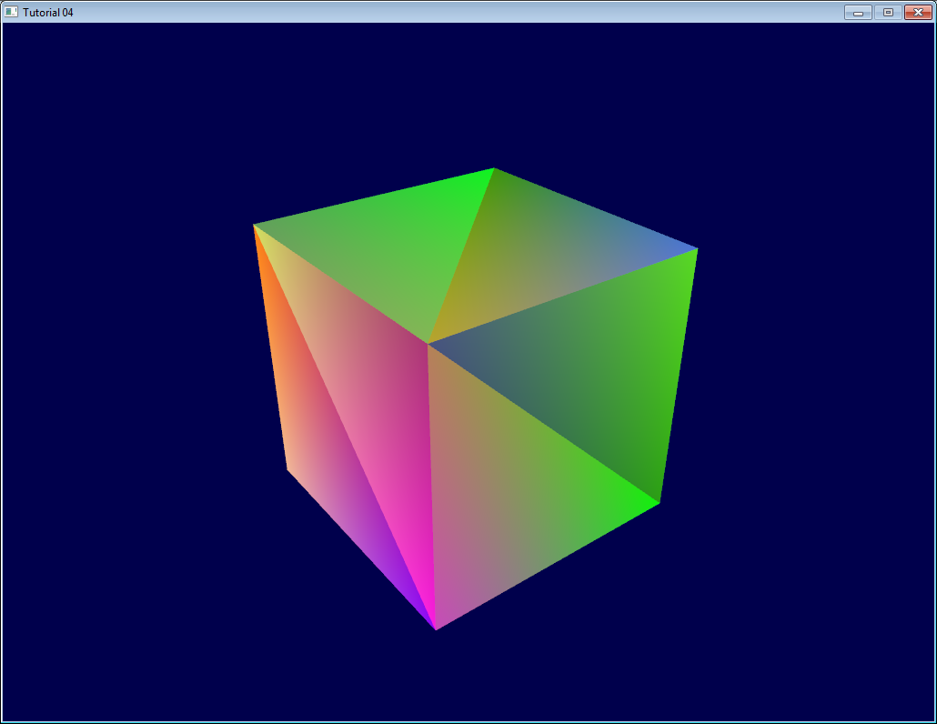
And that’s what we get :
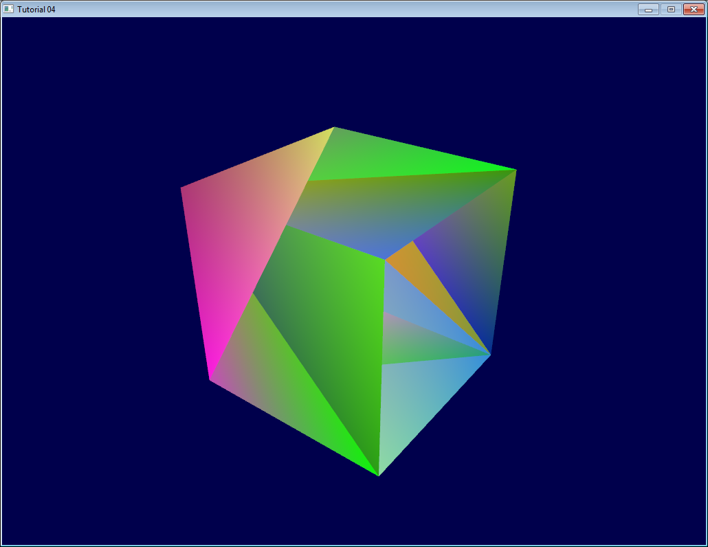
Urgh. Ugly. To understand what happens, here’s what happens when you draw a “far” triangle and a “near” triangle :
Seems OK. Now draw the “far” triangle last :
It overdraws the “near” one, even though it’s supposed to be behind it ! This is what happens with our cube : some faces are supposed to be hidden, but since they are drawn last, they are visible. Let’s call the Z-Buffer to the rescue !
Quick Note 1 : If you don’t see the problem, change your camera position to (4,3,-3)
Quick Note 2 : if “color is like position, it’s an attribute”, why do we need to declare out vec3 fragmentColor; and in vec3 fragmentColor; for the color, and not for the position ? Because the position is actually a bit special : It’s the only thing that is compulsory (or OpenGL wouldn’t know where to draw the triangle !). So in the vertex shader, gl_Position is a “built-in” variable.
The Z-Buffer
The solution to this problem is to store the depth (i.e. “Z”) component of each fragment in a buffer, and each and every time you want to write a fragment, you first check if you should (i.e the new fragment is closer than the previous one).
You can do this yourself, but it’s so much simpler to just ask the hardware to do it itself :
// Enable depth test
glEnable(GL_DEPTH_TEST);
// Accept fragment if it closer to the camera than the former one
glDepthFunc(GL_LESS);
You also need to clear the depth each frame, instead of only the color :
// Clear the screen
glClear(GL_COLOR_BUFFER_BIT | GL_DEPTH_BUFFER_BIT);
And this is enough to solve all your problems.
Exercises
-
Draw the cube AND the triangle, at different locations. You will need to generate 2 MVP matrices, to make 2 draw calls in the main loop, but only 1 shader is required.
-
Generate the color values yourself. Some ideas : At random, so that colors change at each run; Depending on the position of the vertex; a mix of the two; Some other creative idea :) In case you don’t know C, here’s the syntax :
static GLfloat g_color_buffer_data[12*3*3];
for (int v = 0; v < 12*3 ; v++){
    g_color_buffer_data[3*v+0] = your red color here;
    g_color_buffer_data[3*v+1] = your green color here;
    g_color_buffer_data[3*v+2] = your blue color here;
}
- Once you’ve done that, make the colors change each frame. You’ll have to call glBufferData each frame. Make sure the appropriate buffer is bound (glBindBuffer) before !
Tutorial 5 : A Textured Cube
- About UV coordinates
- Loading .BMP images yourself
- Using the texture in OpenGL
- What is filtering and mipmapping, and how to use them
- How to load texture with GLFW
- Compressed Textures
- Conclusion
- Exercices
- References
In this tutorial, you will learn :
- What are UV coordinates
- How to load textures yourself
- How to use them in OpenGL
- What is filtering and mipmapping, and how to use them
- How to load texture more robustly with GLFW
- What the alpha channel is
About UV coordinates
When texturing a mesh, you need a way to tell to OpenGL which part of the image has to be used for each triangle. This is done with UV coordinates.
Each vertex can have, on top of its position, a couple of floats, U and V. These coordinates are used to access the texture, in the following way :

Notice how the texture is distorted on the triangle.
Loading .BMP images yourself
Knowing the BMP file format is not crucial : plenty of libraries can load BMP files for you. But it’s very simple and can help you understand how things work under the hood. So we’ll write a BMP file loader from scratch, so that you know how it works, and never use it again.
Here is the declaration of the loading function :
GLuint loadBMP_custom(const char * imagepath);
so it’s used like this :
GLuint image = loadBMP_custom("./my_texture.bmp");
Let’s see how to read a BMP file, then.
First, we’ll need some data. These variable will be set when reading the file.
// Data read from the header of the BMP file
unsigned char header[54]; // Each BMP file begins by a 54-bytes header
unsigned int dataPos;     // Position in the file where the actual data begins
unsigned int width, height;
unsigned int imageSize;   // = width*height*3
// Actual RGB data
unsigned char * data;
We now have to actually open the file
// Open the file
FILE * file = fopen(imagepath,"rb");
if (!file){printf("Image could not be opened\n"); return 0;}
The first thing in the file is a 54-bytes header. It contains information such as “Is this file really a BMP file?”, the size of the image, the number of bits per pixel, etc. So let’s read this header :
if ( fread(header, 1, 54, file)!=54 ){ // If not 54 bytes read : problem
    printf("Not a correct BMP file\n");
    return false;
}
The header always begins by BM. As a matter of fact, here’s what you get when you open a .BMP file in a hexadecimal editor :
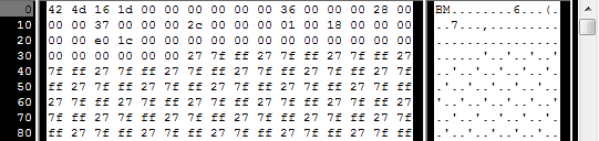
So we have to check that the two first bytes are really ‘B’ and ‘M’ :
if ( header[0]!='B' || header[1]!='M' ){
    printf("Not a correct BMP file\n");
    return 0;
}
Now we can read the size of the image, the location of the data in the file, etc :
// Read ints from the byte array
dataPos    = *(int*)&(header[0x0A]);
imageSize  = *(int*)&(header[0x22]);
width      = *(int*)&(header[0x12]);
height     = *(int*)&(header[0x16]);
We have to make up some info if it’s missing :
// Some BMP files are misformatted, guess missing information
if (imageSize==0)    imageSize=width*height*3; // 3 : one byte for each Red, Green and Blue component
if (dataPos==0)      dataPos=54; // The BMP header is done that way
Now that we know the size of the image, we can allocate some memory to read the image into, and read :
// Create a buffer
data = new unsigned char [imageSize];

// Read the actual data from the file into the buffer
fread(data,1,imageSize,file);

//Everything is in memory now, the file can be closed
fclose(file);
We arrive now at the real OpenGL part. Creating textures is very similar to creating vertex buffers : Create a texture, bind it, fill it, and configure it.
In glTexImage2D, the GL_RGB indicates that we are talking about a 3-component color, and GL_BGR says how exactly it is represented in RAM. As a matter of fact, BMP does not store Red->Green->Blue but Blue->Green->Red, so we have to tell it to OpenGL.
// Create one OpenGL texture
GLuint textureID;
glGenTextures(1, &textureID);

// "Bind" the newly created texture : all future texture functions will modify this texture
glBindTexture(GL_TEXTURE_2D, textureID);

// Give the image to OpenGL
glTexImage2D(GL_TEXTURE_2D, 0,GL_RGB, width, height, 0, GL_BGR, GL_UNSIGNED_BYTE, data);

glTexParameteri(GL_TEXTURE_2D, GL_TEXTURE_MAG_FILTER, GL_NEAREST);
glTexParameteri(GL_TEXTURE_2D, GL_TEXTURE_MIN_FILTER, GL_NEAREST);
We’ll explain those last two lines later. Meanwhile, on the C++-side, you can use your new function to load a texture :
GLuint Texture = loadBMP_custom("uvtemplate.bmp");
Another very important point :** use power-of-two textures !**
- good : 128*128, 256*256, 1024*1024, 2*2…
- bad : 127*128, 3*5, …
- okay but weird : 128*256
Using the texture in OpenGL
We’ll have a look at the fragment shader first. Most of it is straightforward :
#version 330 core

// Interpolated values from the vertex shaders
in vec2 UV;

// Ouput data
out vec3 color;

// Values that stay constant for the whole mesh.
uniform sampler2D myTextureSampler;

void main(){

    // Output color = color of the texture at the specified UV
    color = texture( myTextureSampler, UV ).rgb;
}
Three things :
- The fragment shader needs UV coordinates. Seems fair.
- It also needs a “sampler2D” in order to know which texture to access (you can access several texture in the same shader)
- Finally, accessing a texture is done with texture(), which gives back a (R,G,B,A) vec4. We’ll see about the A shortly.
The vertex shader is simple too, you just have to pass the UVs to the fragment shader :
#version 330 core

// Input vertex data, different for all executions of this shader.
layout(location = 0) in vec3 vertexPosition_modelspace;
layout(location = 1) in vec2 vertexUV;

// Output data ; will be interpolated for each fragment.
out vec2 UV;

// Values that stay constant for the whole mesh.
uniform mat4 MVP;

void main(){

    // Output position of the vertex, in clip space : MVP * position
    gl_Position =  MVP * vec4(vertexPosition_modelspace,1);

    // UV of the vertex. No special space for this one.
    UV = vertexUV;
}
Remember “layout(location = 1) in vec2 vertexUV” from Tutorial 4 ? Well, we’ll have to do the exact same thing here, but instead of giving a buffer (R,G,B) triplets, we’ll give a buffer of (U,V) pairs.
// Two UV coordinatesfor each vertex. They were created with Blender. You'll learn shortly how to do this yourself.
static const GLfloat g_uv_buffer_data[] = {
    0.000059f, 1.0f-0.000004f,
    0.000103f, 1.0f-0.336048f,
    0.335973f, 1.0f-0.335903f,
    1.000023f, 1.0f-0.000013f,
    0.667979f, 1.0f-0.335851f,
    0.999958f, 1.0f-0.336064f,
    0.667979f, 1.0f-0.335851f,
    0.336024f, 1.0f-0.671877f,
    0.667969f, 1.0f-0.671889f,
    1.000023f, 1.0f-0.000013f,
    0.668104f, 1.0f-0.000013f,
    0.667979f, 1.0f-0.335851f,
    0.000059f, 1.0f-0.000004f,
    0.335973f, 1.0f-0.335903f,
    0.336098f, 1.0f-0.000071f,
    0.667979f, 1.0f-0.335851f,
    0.335973f, 1.0f-0.335903f,
    0.336024f, 1.0f-0.671877f,
    1.000004f, 1.0f-0.671847f,
    0.999958f, 1.0f-0.336064f,
    0.667979f, 1.0f-0.335851f,
    0.668104f, 1.0f-0.000013f,
    0.335973f, 1.0f-0.335903f,
    0.667979f, 1.0f-0.335851f,
    0.335973f, 1.0f-0.335903f,
    0.668104f, 1.0f-0.000013f,
    0.336098f, 1.0f-0.000071f,
    0.000103f, 1.0f-0.336048f,
    0.000004f, 1.0f-0.671870f,
    0.336024f, 1.0f-0.671877f,
    0.000103f, 1.0f-0.336048f,
    0.336024f, 1.0f-0.671877f,
    0.335973f, 1.0f-0.335903f,
    0.667969f, 1.0f-0.671889f,
    1.000004f, 1.0f-0.671847f,
    0.667979f, 1.0f-0.335851f
};
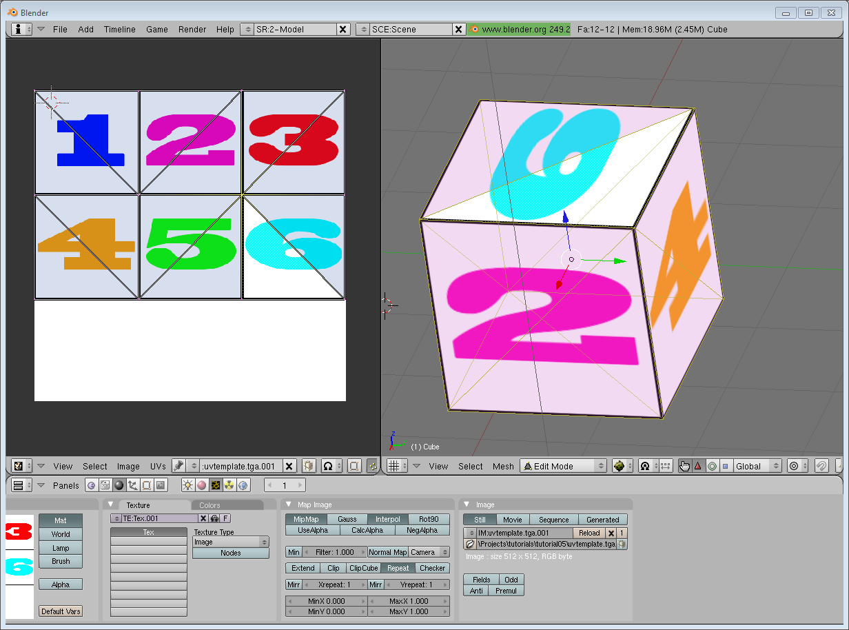
The UV coordinates above correspond to the following model :
The rest is obvious. Generate the buffer, bind it, fill it, configure it, and draw the Vertex Buffer as usual. Just be careful to use 2 as the second parameter (size) of glVertexAttribPointer instead of 3.
This is the result :

and a zoomed-in version :

What is filtering and mipmapping, and how to use them
As you can see in the screenshot above, the texture quality is not that great. This is because in loadBMP_custom, we wrote :
glTexParameteri(GL_TEXTURE_2D, GL_TEXTURE_MAG_FILTER, GL_NEAREST);
glTexParameteri(GL_TEXTURE_2D, GL_TEXTURE_MIN_FILTER, GL_NEAREST);
This means that in our fragment shader, texture() takes the texel that is at the (U,V) coordinates, and continues happily.
There are several things we can do to improve this.
Linear filtering
With linear filtering, texture() also looks at the other texels around, and mixes the colours according to the distance to each center. This avoids the hard edges seen above.

This is much better, and this is used a lot, but if you want very high quality you can also use anisotropic filtering, which is a bit slower.
Anisotropic filtering
This one approximates the part of the image that is really seen through the fragment. For instance, if the following texture is seen from the side, and a little bit rotated, anisotropic filtering will compute the colour contained in the blue rectangle by taking a fixed number of samples (the “anisotropic level”) along its main direction.
Mipmaps
Both linear and anisotropic filtering have a problem. If the texture is seen from far away, mixing only 4 texels won’t be enough. Actually, if your 3D model is so far away than it takes only 1 fragment on screen, ALL the texels of the image should be averaged to produce the final color. This is obviously not done for performance reasons. Instead, we introduce MipMaps :
- At initialisation time, you scale down your image by 2, successively, until you only have a 1x1 image (which effectively is the average of all the texels in the image)
- When you draw a mesh, you select which mipmap is the more appropriate to use given how big the texel should be.
- You sample this mipmap with either nearest, linear or anisotropic filtering
- For additional quality, you can also sample two mipmaps and blend the results.
Luckily, all this is very simple to do, OpenGL does everything for us provided that you ask him nicely :
// When MAGnifying the image (no bigger mipmap available), use LINEAR filtering
glTexParameteri(GL_TEXTURE_2D, GL_TEXTURE_MAG_FILTER, GL_LINEAR);
// When MINifying the image, use a LINEAR blend of two mipmaps, each filtered LINEARLY too
glTexParameteri(GL_TEXTURE_2D, GL_TEXTURE_MIN_FILTER, GL_LINEAR_MIPMAP_LINEAR);
// Generate mipmaps, by the way.
glGenerateMipmap(GL_TEXTURE_2D);
How to load texture with GLFW
Our loadBMP_custom function is great because we made it ourselves, but using a dedicated library is better. GLFW2 can do that too (but only for TGA files, and this feature has been removed in GLFW3, that we now use) :
GLuint loadTGA_glfw(const char * imagepath){

    // Create one OpenGL texture
    GLuint textureID;
    glGenTextures(1, &textureID);

    // "Bind" the newly created texture : all future texture functions will modify this texture
    glBindTexture(GL_TEXTURE_2D, textureID);

    // Read the file, call glTexImage2D with the right parameters
    glfwLoadTexture2D(imagepath, 0);

    // Nice trilinear filtering.
    glTexParameteri(GL_TEXTURE_2D, GL_TEXTURE_WRAP_S, GL_REPEAT);
    glTexParameteri(GL_TEXTURE_2D, GL_TEXTURE_WRAP_T, GL_REPEAT);
    glTexParameteri(GL_TEXTURE_2D, GL_TEXTURE_MAG_FILTER, GL_LINEAR);
    glTexParameteri(GL_TEXTURE_2D, GL_TEXTURE_MIN_FILTER, GL_LINEAR_MIPMAP_LINEAR);
    glGenerateMipmap(GL_TEXTURE_2D);

    // Return the ID of the texture we just created
    return textureID;
}
Compressed Textures
At this point, you’re probably wondering how to load JPEG files instead of TGA.
Short answer : don’t. GPUs can’t understand JPEG. So you’ll compress your original image in JPEG, and decompress it so that the GPU can understand it. You’re back to raw images, but you lost image quality while compressing to JPEG.
There’s a better option.
Creating compressed textures
- Download The Compressonator, an AMD tool
- Load a Power-Of-Two texture in it
- Generate mipmaps so that you won’t have to do it on runtime
- Compress it in DXT1, DXT3 or in DXT5 (more about the differences between the various formats on Wikipedia) :
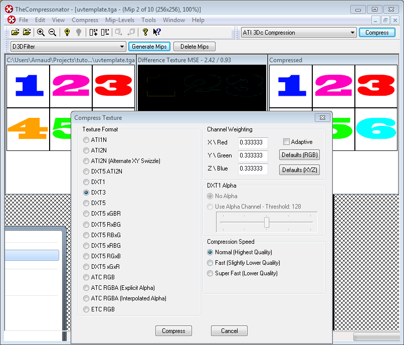
- Export it as a .DDS file.
At this point, your image is compressed in a format that is directly compatible with the GPU. Whenever calling texture() in a shader, it will uncompress it on-the-fly. This can seem slow, but since it takes a LOT less memory, less data needs to be transferred. But memory transfers are expensive; and texture decompression is free (there is dedicated hardware for that). Typically, using texture compression yields a 20% increase in performance. So you save on performance and memory, at the expense of reduced quality.
Using the compressed texture
Let’s see how to load the image. It’s very similar to the BMP code, except that the header is organized differently :
GLuint loadDDS(const char * imagepath){

    unsigned char header[124];

    FILE *fp;

    /* try to open the file */
    fp = fopen(imagepath, "rb");
    if (fp == NULL)
        return 0;

    /* verify the type of file */
    char filecode[4];
    fread(filecode, 1, 4, fp);
    if (strncmp(filecode, "DDS ", 4) != 0) {
        fclose(fp);
        return 0;
    }

    /* get the surface desc */
    fread(&header, 124, 1, fp);

    unsigned int height      = *(unsigned int*)&(header[8 ]);
    unsigned int width         = *(unsigned int*)&(header[12]);
    unsigned int linearSize     = *(unsigned int*)&(header[16]);
    unsigned int mipMapCount = *(unsigned int*)&(header[24]);
    unsigned int fourCC      = *(unsigned int*)&(header[80]);
After the header is the actual data : all the mipmap levels, successively. We can read them all in one batch :
    unsigned char * buffer;
    unsigned int bufsize;
    /* how big is it going to be including all mipmaps? */
    bufsize = mipMapCount > 1 ? linearSize * 2 : linearSize;
    buffer = (unsigned char*)malloc(bufsize * sizeof(unsigned char));
    fread(buffer, 1, bufsize, fp);
    /* close the file pointer */
    fclose(fp);
Here we’ll deal with 3 different formats : DXT1, DXT3 and DXT5. We need to convert the “fourCC” flag into a value that OpenGL understands.
    unsigned int components  = (fourCC == FOURCC_DXT1) ? 3 : 4;
    unsigned int format;
    switch(fourCC)
    {
    case FOURCC_DXT1:
        format = GL_COMPRESSED_RGBA_S3TC_DXT1_EXT;
        break;
    case FOURCC_DXT3:
        format = GL_COMPRESSED_RGBA_S3TC_DXT3_EXT;
        break;
    case FOURCC_DXT5:
        format = GL_COMPRESSED_RGBA_S3TC_DXT5_EXT;
        break;
    default:
        free(buffer);
        return 0;
    }
Creating the texture is done as usual :
    // Create one OpenGL texture
    GLuint textureID;
    glGenTextures(1, &textureID);

    // "Bind" the newly created texture : all future texture functions will modify this texture
    glBindTexture(GL_TEXTURE_2D, textureID);
And now, we just have to fill each mipmap one after another :
    unsigned int blockSize = (format == GL_COMPRESSED_RGBA_S3TC_DXT1_EXT) ? 8 : 16;
    unsigned int offset = 0;

    /* load the mipmaps */
    for (unsigned int level = 0; level < mipMapCount && (width || height); ++level)
    {
        unsigned int size = ((width+3)/4)*((height+3)/4)*blockSize;
        glCompressedTexImage2D(GL_TEXTURE_2D, level, format, width, height,
            0, size, buffer + offset);

        offset += size;
        width  /= 2;
        height /= 2;
    }
    free(buffer);

    return textureID;
Inversing the UVs
DXT compression comes from the DirectX world, where the V texture coordinate is inversed compared to OpenGL. So if you use compressed textures, you’ll have to use ( coord.u, 1.0-coord.v) to fetch the correct texel. You can do this whenever you want : in your export script, in your loader, in your shader…
Conclusion
You just learnt to create, load and use textures in OpenGL.
In general, you should only use compressed textures, since they are smaller to store, almost instantaneous to load, and faster to use; the main drawback it that you have to convert your images through The Compressonator (or any similar tool)
Exercices
- The DDS loader is implemented in the source code, but not the texture coordinate modification. Change the code at the appropriate place to display the cube correctly.
- Experiment with the various DDS formats. Do they give different result ? Different compression ratios ?
- Try not to generate mipmaps in The Compressonator. What is the result ? Give 3 different ways to fix this.
References
- Using texture compression in OpenGL , Sébastien Domine, NVIDIA
Tutorial 6 : Keyboard and Mouse
Welcome for our 6th tutorial !
We will now learn how to use the mouse and the keyboard to move the camera just like in a FPS.
The interface
Since this code will be re-used throughout the tutorials, we will put the code in a separate file : common/controls.cpp, and declare the functions in common/controls.hpp so that tutorial06.cpp knows about them.
The code of tutorial06.cpp doesn’t change much from the previous tutorial. The major modification is that instead of computing the MVP matrix once, we now have to do it every frame. So let’s move this code inside the main loop :
do{

    // ...

    // Compute the MVP matrix from keyboard and mouse input
    computeMatricesFromInputs();
    glm::mat4 ProjectionMatrix = getProjectionMatrix();
    glm::mat4 ViewMatrix = getViewMatrix();
    glm::mat4 ModelMatrix = glm::mat4(1.0);
    glm::mat4 MVP = ProjectionMatrix * ViewMatrix * ModelMatrix;

    // ...
}
This code needs 3 new functions :
- computeMatricesFromInputs() reads the keyboard and mouse and computes the Projection and View matrices. This is where all the magic happens.
- getProjectionMatrix() just returns the computed Projection matrix.
- getViewMatrix() just returns the computed View matrix.
This is just one way to do it, of course. If you don’t like these functions, go ahead and change them.
Let’s see what’s inside controls.cpp.
The actual code
We’ll need a few variables.
// position
glm::vec3 position = glm::vec3( 0, 0, 5 );
// horizontal angle : toward -Z
float horizontalAngle = 3.14f;
// vertical angle : 0, look at the horizon
float verticalAngle = 0.0f;
// Initial Field of View
float initialFoV = 45.0f;

float speed = 3.0f; // 3 units / second
float mouseSpeed = 0.005f;
FoV is the level of zoom. 80° = very wide angle, huge deformations. 60° - 45° : standard. 20° : big zoom.
We will first recompute position, horizontalAngle, verticalAngle and FoV according to the inputs, and then compute the View and Projection matrices from position, horizontalAngle, verticalAngle and FoV.
Orientation
Reading the mouse position is easy :
// Get mouse position
int xpos, ypos;
glfwGetMousePos(&xpos, &ypos);
but we have to take care to put the cursor back to the center of the screen, or it will soon go outside the window and you won’t be able to move anymore.
// Reset mouse position for next frame
glfwSetMousePos(1024/2, 768/2);
Notice that this code assumes that the window is 1024*768, which of course is not necessarily the case. You can use glfwGetWindowSize if you want, too.
We can now compute our viewing angles :
// Compute new orientation
horizontalAngle += mouseSpeed * deltaTime * float(1024/2 - xpos );
verticalAngle   += mouseSpeed * deltaTime * float( 768/2 - ypos );
Let’s read this from right to left :
- 1024/2 - xpos means : how far is the mouse from the center of the window ? The bigger this value, the more we want to turn.
- float(…) converts it to a floating-point number so that the multiplication goes well.
- mouseSpeed is just there to speed up or slow down the rotations. Fine-tune this at will, or let the user choose it.
- += : If you didn’t move the mouse, 1024/2-xpos will be 0, and horizontalAngle+=0 doesn’t change horizontalAngle. If you had a “=” instead, you would be forced back to your original orientation each frame, which isn’t good.
We can now compute a vector that represents, in World Space, the direction in which we’re looking
// Direction : Spherical coordinates to Cartesian coordinates conversion
glm::vec3 direction(
    cos(verticalAngle) * sin(horizontalAngle),
    sin(verticalAngle),
    cos(verticalAngle) * cos(horizontalAngle)
);
This is a standard computation, but if you don’t know about cosine and sinus, here’s a short explanation :

The formula above is just the generalisation to 3D.
Now we want to compute the “up” vector reliably. Notice that “up” isn’t always towards +Y : if you look down, for instance, the “up” vector will be in fact horizontal. Here is an example of to cameras with the same position, the same target, but a different up:
In our case, the only constant is that the vector goes to the right of the camera is always horizontal. You can check this by putting your arm horizontal, and looking up, down, in any direction. So let’s define the “right” vector : its Y coordinate is 0 since it’s horizontal, and its X and Z coordinates are just like in the figure above, but with the angles rotated by 90°, or Pi/2 radians.
// Right vector
glm::vec3 right = glm::vec3(
    sin(horizontalAngle - 3.14f/2.0f),
    0,
    cos(horizontalAngle - 3.14f/2.0f)
);
We have a “right” vector and a “direction”, or “front” vector. The “up” vector is a vector that is perpendicular to these two. A useful mathematical tool makes this very easy : the cross product.
// Up vector : perpendicular to both direction and right
glm::vec3 up = glm::cross( right, direction );
To remember what the cross product does, it’s very simple. Just recall the Right Hand Rule from Tutorial 3. The first vector is the thumb; the second is the index; and the result is the middle finger. It’s very handy.
Position
The code is pretty straightforward. By the way, I used the up/down/right/left keys instead of the awsd because on my azerty keyboard, awsd is actually zqsd. And it’s also different with qwerZ keyboards, let alone korean keyboards. I don’t even know what layout korean people have, but I guess it’s also different.
// Move forward
if (glfwGetKey( GLFW_KEY_UP ) == GLFW_PRESS){
    position += direction * deltaTime * speed;
}
// Move backward
if (glfwGetKey( GLFW_KEY_DOWN ) == GLFW_PRESS){
    position -= direction * deltaTime * speed;
}
// Strafe right
if (glfwGetKey( GLFW_KEY_RIGHT ) == GLFW_PRESS){
    position += right * deltaTime * speed;
}
// Strafe left
if (glfwGetKey( GLFW_KEY_LEFT ) == GLFW_PRESS){
    position -= right * deltaTime * speed;
}
The only special thing here is the deltaTime. You don’t want to move from 1 unit each frame for a simple reason :
- If you have a fast computer, and you run at 60 fps, you’d move of 60*speed units in 1 second
- If you have a slow computer, and you run at 20 fps, you’d move of 20*speed units in 1 second
Since having a better computer is not an excuse for going faster, you have to scale the distance by the “time since the last frame”, or “deltaTime”.
- If you have a fast computer, and you run at 60 fps, you’d move of 1/60 * speed units in 1 frame, so 1*speed in 1 second.
- If you have a slow computer, and you run at 20 fps, you’d move of 1/20 * speed units in 1 second, so 1*speed in 1 second.
which is much better. deltaTime is very simple to compute :
double currentTime = glfwGetTime();
float deltaTime = float(currentTime - lastTime);
Field Of View
For fun, we can also bind the wheel of the mouse to the Field Of View, so that we can have a cheap zoom :
float FoV = initialFoV - 5 * glfwGetMouseWheel();
Computing the matrices
Computing the matrices is now straightforward. We use the exact same functions than before, but with our new parameters.
// Projection matrix : 45° Field of View, 4:3 ratio, display range : 0.1 unit <-> 100 units
ProjectionMatrix = glm::perspective(glm::radians(FoV), 4.0f / 3.0f, 0.1f, 100.0f);
// Camera matrix
ViewMatrix = glm::lookAt(
position, // Camera is here
position+direction, // and looks here : at the same position, plus "direction"
up // Head is up (set to 0,-1,0 to look upside-down)
);
Results
Backface Culling
Now that you can freely move around, you’ll notice that if you go inside the cube, polygons are still displayed. This can seem obvious, but this remark actually opens an opportunity for optimisation. As a matter of fact, in a usual application, you are never inside a cube.
The idea is to let the GPU check if the camera is behind, or in front of, the triangle. If it’s in front, display the triangle; if it’s behind, and the mesh is closed, and we’re not inside the mesh, then there will be another triangle in front of it, and nobody will notice anything, except that everything will be faster : 2 times less triangles on average !
The best thing is that it’s very easy to check this. The GPU computes the normal of the triangle (using the cross product, remember ?) and checks whether this normal is oriented towards the camera or not.
This comes at a cost, unfortunately : the orientation of the triangle is implicit. This means that is you invert two vertices in your buffer, you’ll probably end up with a hole. But it’s generally worth the little additional work. Often, you just have to click “invert normals” in your 3D modeler (which will, in fact, invert vertices, and thus normals) and everything is just fine.
Enabling backface culling is a breeze :
// Cull triangles which normal is not towards the camera
glEnable(GL_CULL_FACE);
Exercices
- Restrict verticalAngle so that you can’t go upside-down
- Create a camera that rotates around the object ( position = ObjectCenter + ( radius * cos(time), height, radius * sin(time) ) ); bind the radius/height/time to the keyboard/mouse, or whatever
- Have fun !
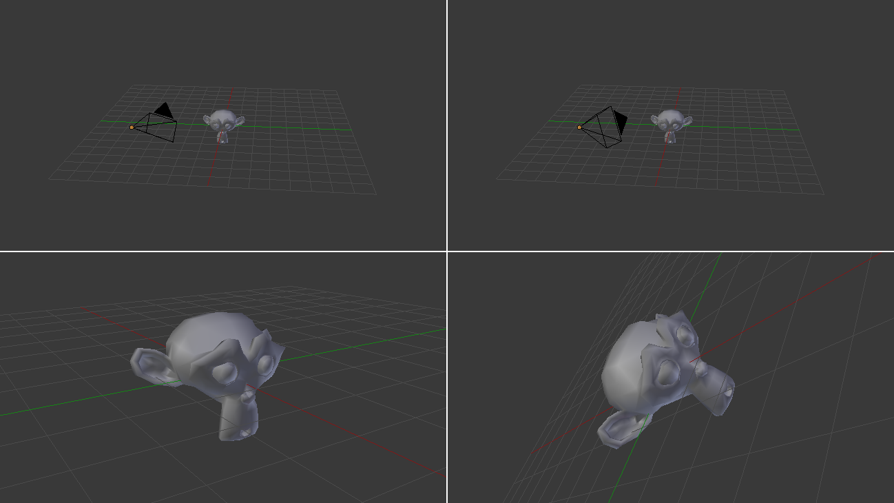
Tutorial 7 : Model loading
Until now, we hardcoded our cube directly in the source code. I’m sure you will agree that this was cumbersome and not very handy.
In this tutorial we will learn how to load 3D meshes from files. We will do this just like we did for the textures : we will write a tiny, very limited loader, and I’ll give you some pointers to actual libraries that can do this better that us.
To keep this tutorial as simple as possible, we’ll use the OBJ file format, which is both very simple and very common. And once again, to keep things simple, we will only deal with OBJ files with 1 UV coordinate and 1 normal per vertex (you don’t have to know what a normal is right now).
Loading the OBJ
Our function, located in common/objloader.cpp and declared in common/objloader.hpp, will have the following signature :
bool loadOBJ(
    const char * path,
    std::vector < glm::vec3 > & out_vertices,
    std::vector < glm::vec2 > & out_uvs,
    std::vector < glm::vec3 > & out_normals
)
We want loadOBJ to read the file “path”, write the data in out_vertices/out_uvs/out_normals, and return false if something went wrong. std::vector is the C++ way to declare an array of glm::vec3 which size can be modified at will: it has nothing to do with a mathematical vector. Just an array, really. And finally, the & means that function will be able to modify the std::vectors.
Example OBJ file
An OBJ file looks more or less like this :
# Blender3D v249 OBJ File: untitled.blend
# www.blender3d.org
mtllib cube.mtl
v 1.000000 -1.000000 -1.000000
v 1.000000 -1.000000 1.000000
v -1.000000 -1.000000 1.000000
v -1.000000 -1.000000 -1.000000
v 1.000000 1.000000 -1.000000
v 0.999999 1.000000 1.000001
v -1.000000 1.000000 1.000000
v -1.000000 1.000000 -1.000000
vt 0.748573 0.750412
vt 0.749279 0.501284
vt 0.999110 0.501077
vt 0.999455 0.750380
vt 0.250471 0.500702
vt 0.249682 0.749677
vt 0.001085 0.750380
vt 0.001517 0.499994
vt 0.499422 0.500239
vt 0.500149 0.750166
vt 0.748355 0.998230
vt 0.500193 0.998728
vt 0.498993 0.250415
vt 0.748953 0.250920
vn 0.000000 0.000000 -1.000000
vn -1.000000 -0.000000 -0.000000
vn -0.000000 -0.000000 1.000000
vn -0.000001 0.000000 1.000000
vn 1.000000 -0.000000 0.000000
vn 1.000000 0.000000 0.000001
vn 0.000000 1.000000 -0.000000
vn -0.000000 -1.000000 0.000000
usemtl Material_ray.png
s off
f 5/1/1 1/2/1 4/3/1
f 5/1/1 4/3/1 8/4/1
f 3/5/2 7/6/2 8/7/2
f 3/5/2 8/7/2 4/8/2
f 2/9/3 6/10/3 3/5/3
f 6/10/4 7/6/4 3/5/4
f 1/2/5 5/1/5 2/9/5
f 5/1/6 6/10/6 2/9/6
f 5/1/7 8/11/7 6/10/7
f 8/11/7 7/12/7 6/10/7
f 1/2/8 2/9/8 3/13/8
f 1/2/8 3/13/8 4/14/8
So :
#is a comment, just like // in C++- usemtl and mtllib describe the look of the model. We won’t use this in this tutorial.
- v is a vertex
- vt is the texture coordinate of one vertex
- vn is the normal of one vertex
- f is a face
v, vt and vn are simple to understand. f is more tricky. So, for f 8/11/7 7/12/7 6/10/7 :
- 8/11/7 describes the first vertex of the triangle
- 7/12/7 describes the second vertex of the triangle
- 6/10/7 describes the third vertex of the triangle (duh)
- For the first vertex, 8 says which vertex to use. So in this case, -1.000000 1.000000 -1.000000 (index start to 1, not to 0 like in C++)
- 11 says which texture coordinate to use. So in this case, 0.748355 0.998230
- 7 says which normal to use. So in this case, 0.000000 1.000000 -0.000000
These numbers are called indices. It’s handy because if several vertices share the same position, you just have to write one “v” in the file, and use it several times. This saves memory.
The bad news is that OpenGL can’t be told to use one index for the position, another for the texture, and another for the normal. So the approach I took for this tutorial is to make a standard, non-indexed mesh, and deal with indexing later, in Tutorial 9, which will explain how to work around this.
Creating an OBJ file in Blender
Since our toy loader will be severely limited, we have to be extra careful to set the right options when exporting the file. Here’s how it should look in Blender :
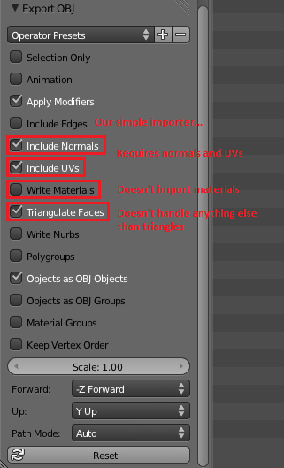
Reading the file
Ok, down with the actual code. We need some temporary variables in which we will store the contents of the .obj :
std::vector< unsigned int > vertexIndices, uvIndices, normalIndices;
std::vector< glm::vec3 > temp_vertices;
std::vector< glm::vec2 > temp_uvs;
std::vector< glm::vec3 > temp_normals;
Since Tutorial 5 : A Textured Cube, you know how to open a file :
FILE * file = fopen(path, "r");
if( file == NULL ){
    printf("Impossible to open the file !\n");
    return false;
}
Let’s read this file until the end :
while( 1 ){

    char lineHeader[128];
    // read the first word of the line
    int res = fscanf(file, "%s", lineHeader);
    if (res == EOF)
        break; // EOF = End Of File. Quit the loop.

    // else : parse lineHeader
(notice that we assume that the first word of a line won’t be longer than 128, which is a very silly assumption. But for a toy parser, it’s all right)
Let’s deal with the vertices first :
if ( strcmp( lineHeader, "v" ) == 0 ){
    glm::vec3 vertex;
    fscanf(file, "%f %f %f\n", &vertex.x, &vertex.y, &vertex.z );
    temp_vertices.push_back(vertex);
i.e : If the first word of the line is “v”, then the rest has to be 3 floats, so create a glm::vec3 out of them, and add it to the vector.
}else if ( strcmp( lineHeader, "vt" ) == 0 ){
    glm::vec2 uv;
    fscanf(file, "%f %f\n", &uv.x, &uv.y );
    temp_uvs.push_back(uv);
i.e if it’s not a “v” but a “vt”, then the rest has to be 2 floats, so create a glm::vec2 and add it to the vector.
same thing for the normals :
}else if ( strcmp( lineHeader, "vn" ) == 0 ){
    glm::vec3 normal;
    fscanf(file, "%f %f %f\n", &normal.x, &normal.y, &normal.z );
    temp_normals.push_back(normal);
And now the “f”, which is more difficult :
}else if ( strcmp( lineHeader, "f" ) == 0 ){
    std::string vertex1, vertex2, vertex3;
    unsigned int vertexIndex[3], uvIndex[3], normalIndex[3];
    int matches = fscanf(file, "%d/%d/%d %d/%d/%d %d/%d/%d\n", &vertexIndex[0], &uvIndex[0], &normalIndex[0], &vertexIndex[1], &uvIndex[1], &normalIndex[1], &vertexIndex[2], &uvIndex[2], &normalIndex[2] );
    if (matches != 9){
        printf("File can't be read by our simple parser : ( Try exporting with other options\n");
        return false;
    }
    vertexIndices.push_back(vertexIndex[0]);
    vertexIndices.push_back(vertexIndex[1]);
    vertexIndices.push_back(vertexIndex[2]);
    uvIndices    .push_back(uvIndex[0]);
    uvIndices    .push_back(uvIndex[1]);
    uvIndices    .push_back(uvIndex[2]);
    normalIndices.push_back(normalIndex[0]);
    normalIndices.push_back(normalIndex[1]);
    normalIndices.push_back(normalIndex[2]);
This code is in fact very similar to the previous one, except that there is more data to read.
Processing the data
So what we did there was simply to change the “shape” of the data. We had a string, we now have a set of std::vectors. But it’s not enough, we have to put this into a form that OpenGL likes. Namely, removing the indexes and have plain glm::vec3 instead. This operation is called indexing.
We go through each vertex ( each v/vt/vn ) of each triangle ( each line with a “f” ) :
    // For each vertex of each triangle
    for( unsigned int i=0; i<vertexIndices.size(); i++ ){
the index to the vertex position is vertexIndices[i] :
unsigned int vertexIndex = vertexIndices[i];
so the position is temp_vertices[ vertexIndex-1 ] (there is a -1 because C++ indexing starts at 0 and OBJ indexing starts at 1, remember ?) :
glm::vec3 vertex = temp_vertices[ vertexIndex-1 ];
And this makes the position of our new vertex
out_vertices.push_back(vertex);
The same is applied for UVs and normals, and we’re done !
Using the loaded data
Once we’ve got this, almost nothing changes. Instead of declaring our usual static const GLfloat g_vertex_buffer_data[] = {…}, you declare a std::vector vertices instead (same thing for UVS and normals). You call loadOBJ with the right parameters :
// Read our .obj file
std::vector< glm::vec3 > vertices;
std::vector< glm::vec2 > uvs;
std::vector< glm::vec3 > normals; // Won't be used at the moment.
bool res = loadOBJ("cube.obj", vertices, uvs, normals);
and give your vectors to OpenGL instead of your arrays :
glBufferData(GL_ARRAY_BUFFER, vertices.size() * sizeof(glm::vec3), &vertices[0], GL_STATIC_DRAW);
And that’s it !
Results
Sorry for the lame texture, I’m NOT a good artist :( Any contribution welcome !
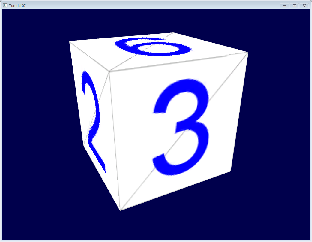
Other formats/loaders
This tiny loader should give you enough to get started, but won’t want to use this in real life. Have a look at our Useful Links & Tools page for some tools you can use. Note, however, that you’d better wait for tutorial 9 before *actually *trying to use them.
Tutorial 8 : Basic shading
In this 8th tutorial, we will learn how to do some basic shading. This includes :
- Beeing more bright when closer to a light source
- Having highlights when looking in the reflection of a light (specular lighting)
- Beeing darker when light is not directly towards the model (diffuse lighting)
- Cheating a lot (ambient lighting)
This does NOT include :
- Shadows. This is a broad topic that deserves its own tutorial(s)
- Mirror-like reflections (this includes water)
- Any sophisticated light-matter interaction like subsurface scattering (like wax)
- Anisotrophic materials (like brushed metal)
- Physically based shading, which tries to mimic the reality closely
- Ambient Occlusion (it’s darker in a cave)
- Color Bleeding (a red carpet will make a white ceiling a litte bit red)
- Transparency
- Any kind of Global Illumination whatsoever (it’s the name that regroups all previous ones)
In a word : Basic.
Normals
During the last few tutorials you’ve been dealing with normal without really knowing what they were.
Triangle normals
The normal of a plane is a vector of length 1 that is perpendicular to this plane.
The normal of a triangle is a vector of length 1 that is perpendicular to this triangle. It is easily computed by taking the cross product of two of its edges (the cross product of a and b produces a vector that is perpendicular to both a and b, remember ?), and normalized : its length is brought back to 1. In pseudo-code :
triangle ( v1, v2, v3 )
edge1 = v2-v1
edge2 = v3-v1
triangle.normal = cross(edge1, edge2).normalize()
Don’t mix up normal and normalize(). Normalize() divides a vector (any vector, not necessarily a normal) by its length so that its new length is 1. normal is just the name for some vectors that happen to represent, well, a normal.
Vertex normals
By extension, we call the normal of a vertex the combination of the normals of the surroundings triangles. This is handy because in vertex shaders, we deal with vertices, not triangles, so it’s better to have information on the vertex. And any way, we can’t have information on triangles in OpenGL. In pseudo-code :
vertex v1, v2, v3, ....
triangle tr1, tr2, tr3 // all share vertex v1
v1.normal = normalize( tr1.normal + tr2.normal + tr3.normal )
Using vertex normals in OpenGL
To use normals in OpenGL, it’s very easy. A normal is an attribute of a vertex, just like its position, its color, its UV coordinates… so just do the usual stuff. Our loadOBJ function from Tutorial 7 already reads them from the OBJ file.
GLuint normalbuffer;
 glGenBuffers(1, &normalbuffer);
 glBindBuffer(GL_ARRAY_BUFFER, normalbuffer);
 glBufferData(GL_ARRAY_BUFFER, normals.size() * sizeof(glm::vec3), &normals[0], GL_STATIC_DRAW);
and
 // 3rd attribute buffer : normals
 glEnableVertexAttribArray(2);
 glBindBuffer(GL_ARRAY_BUFFER, normalbuffer);
 glVertexAttribPointer(
     2,                                // attribute
     3,                                // size
     GL_FLOAT,                         // type
     GL_FALSE,                         // normalized?
     0,                                // stride
     (void*)0                          // array buffer offset
 );
and this is enough to get us started.
The Diffuse part
The importance of the surface normal
When light hits an object, an important fraction of it is reflected in all directions. This is the “diffuse component”. (We’ll see what happens with the other fraction soon)
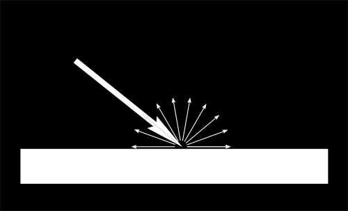
When a certain flux of light arrives at the surface, this surface is illuminated differently according to the angle at which the light arrives.
If the light is perpendicular to the surface, it is concentrated on a small surface. If it arrives at a gazing angle, the same quantity of light spreads on a greater surface :
This means that each point of the surface will look darker with gazing light (but remember, more points will be illuminated, so the total quantity of light will remain the same)
This means that when we compute the colour of a pixel, the angle between the incoming light and the surface normal matters. We thus have :
// Cosine of the angle between the normal and the light direction,
// clamped above 0
//  - light is at the vertical of the triangle -> 1
//  - light is perpendicular to the triangle -> 0
float cosTheta = dot( n,l );

color = LightColor * cosTheta;
In this code, n is the surface normal and l is the unit vector that goes from the surface to the light (and not the contrary, even if it’s non inuitive. It makes the math easier).
Beware of the sign
Something is missing in the formula of our cosTheta. If the light is behind the triangle, n and l will be opposed, so n.l will be negative. This would mean that colour = someNegativeNumber, which doesn’t mean much. So we have to clamp cosTheta to 0 :
// Cosine of the angle between the normal and the light direction,
// clamped above 0
//  - light is at the vertical of the triangle -> 1
//  - light is perpendicular to the triangle -> 0
//  - light is behind the triangle -> 0
float cosTheta = clamp( dot( n,l ), 0,1 );

color = LightColor * cosTheta;
Material Color
Of course, the output colour also depends on the colour of the material. In this image, the white light is made out of green, red and blue light. When colliding with the red material, green and blue light is absorbed, and only the red remains.
We can model this by a simple multiplication :
color = MaterialDiffuseColor * LightColor * cosTheta;
Modeling the light
We will first assume that we have a punctual light that emits in all directions in space, like a candle.
With such a light, the luminous flux that our surface will receive will depend on its distance to the light source: the further away, the less light. In fact, the amount of light will diminish with the square of the distance :
color = MaterialDiffuseColor * LightColor * cosTheta / (distance*distance);
Lastly, we need another parameter to control the power of the light. This could be encoded into LightColor (and we will in a later tutorial), but for now let’s just have a color (e.g. white) and a power (e.g. 60 Watts).
color = MaterialDiffuseColor * LightColor * LightPower * cosTheta / (distance*distance);
Putting it all together
For this code to work, we need a handful of parameters (the various colours and powers) and some more code.
MaterialDiffuseColor is simply fetched from the texture.
LightColor and LightPower are set in the shader through GLSL uniforms.
cosTheta depends on n and l. We can express them in any space provided it’s the same for both. We choose the camera space because it’s easy to compute the light’s position in this space :
// Normal of the computed fragment, in camera space
 vec3 n = normalize( Normal_cameraspace );
 // Direction of the light (from the fragment to the light)
 vec3 l = normalize( LightDirection_cameraspace );
with Normal_cameraspace and LightDirection_cameraspace computed in the Vertex shader and passed to the fragment shader :
// Output position of the vertex, in clip space : MVP * position
gl_Position =  MVP * vec4(vertexPosition_modelspace,1);

// Position of the vertex, in worldspace : M * position
Position_worldspace = (M * vec4(vertexPosition_modelspace,1)).xyz;

// Vector that goes from the vertex to the camera, in camera space.
// In camera space, the camera is at the origin (0,0,0).
vec3 vertexPosition_cameraspace = ( V * M * vec4(vertexPosition_modelspace,1)).xyz;
EyeDirection_cameraspace = vec3(0,0,0) - vertexPosition_cameraspace;

// Vector that goes from the vertex to the light, in camera space. M is ommited because it's identity.
vec3 LightPosition_cameraspace = ( V * vec4(LightPosition_worldspace,1)).xyz;
LightDirection_cameraspace = LightPosition_cameraspace + EyeDirection_cameraspace;

// Normal of the the vertex, in camera space
Normal_cameraspace = ( V * M * vec4(vertexNormal_modelspace,0)).xyz; // Only correct if ModelMatrix does not scale the model ! Use its inverse transpose if not.
This code can seem impressive but it’s nothing we didn’t learn in Tutorial 3 : Matrices. I paid attention to write the name of the space in each vector’s name, so that keeping track of what is happening is much easier. You should do that, too.
M and V are the Model and View matrices, which are passed to the shader in the exact same way as MVP.
Time for work
You’ve got everything you need to code a diffuse lighting. Go ahead, and learn the hard way :)
Result
With only the Diffuse component, we have the following result (sorry for the lame texture again) :
It’s better than before, but there is still much missing. In particular, the back of Suzanne is completely black since we used clamp().
The Ambient component
The Ambient component is the biggest cheat ever.
We expect the back of Suzanne to be receive more light because in real life, the lamp would light the wall behind it, which would in turn (slightly less) light the back of the object.
This is awfully expensive to compute.
So the usual hack is to simply fake some light. In fact, is simply makes the 3D model *emit *light so that it doesn’t appear completely black.
This can be done this way :
vec3 MaterialAmbientColor = vec3(0.1,0.1,0.1) * MaterialDiffuseColor;
color =
 // Ambient : simulates indirect lighting
 MaterialAmbientColor +
 // Diffuse : "color" of the object
 MaterialDiffuseColor * LightColor * LightPower * cosTheta / (distance*distance) ;
Let’s see what it gives
Results
Ok so that’s a little bit better. You can adjust the (0.1, 0.1, 0.1) if you want better results.
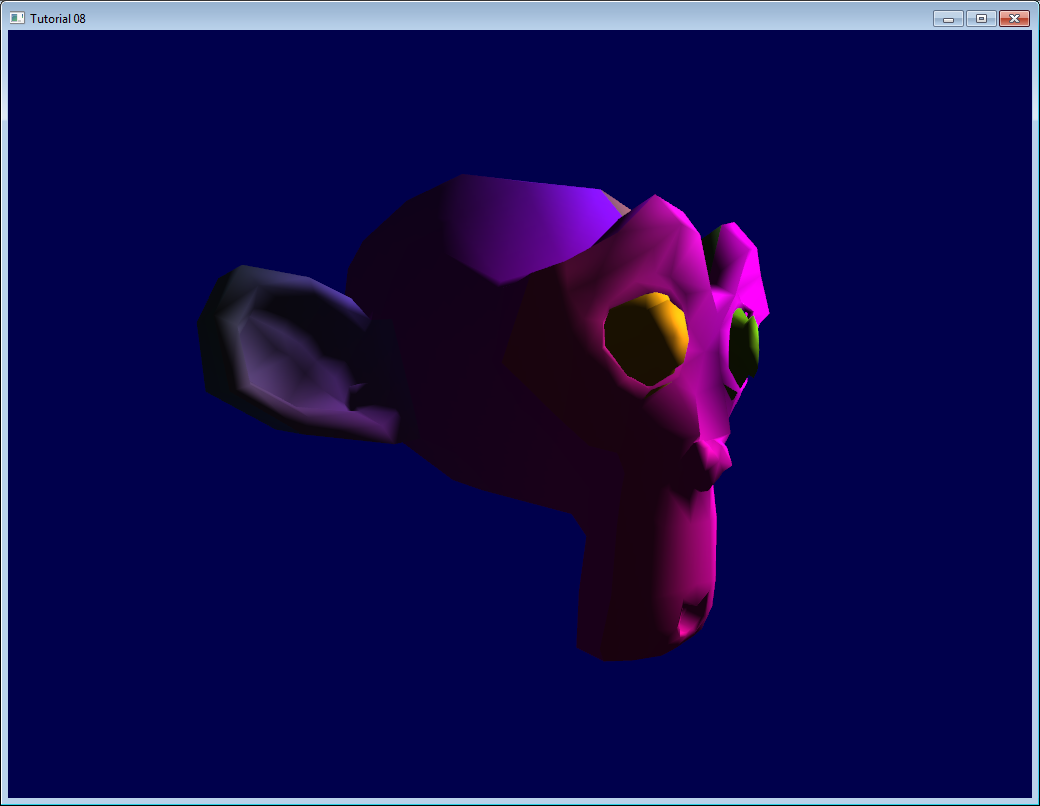
The Specular component
The other part of light that is reflected is reflected mostly in the direction that is the reflection of the light on the surface. This is the specular component.
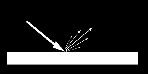
As you can see in the image, it forms a kind of lobe. In extreme cases, the diffuse component can be null, the lobe can be very very very narrow (all the light is reflected in a single direction) and you get a mirror.
(we can indeed tweak the parameters to get a mirror, but in our case, the only thing we take into account in this mirror is the lamp. So this would make for a weird mirror)
// Eye vector (towards the camera)
vec3 E = normalize(EyeDirection_cameraspace);
// Direction in which the triangle reflects the light
vec3 R = reflect(-l,n);
// Cosine of the angle between the Eye vector and the Reflect vector,
// clamped to 0
//  - Looking into the reflection -> 1
//  - Looking elsewhere -> < 1
float cosAlpha = clamp( dot( E,R ), 0,1 );

color =
    // Ambient : simulates indirect lighting
    MaterialAmbientColor +
    // Diffuse : "color" of the object
    MaterialDiffuseColor * LightColor * LightPower * cosTheta / (distance*distance) ;
    // Specular : reflective highlight, like a mirror
    MaterialSpecularColor * LightColor * LightPower * pow(cosAlpha,5) / (distance*distance);
R is the direction in which the light reflects. E is the inverse direction of the eye (just like we did for “l”); If the angle between these two is little, it means we are looking straight into the reflection.
pow(cosAlpha,5) is used to control the width of the specular lobe. Increase 5 to get a thinner lobe.
Final result
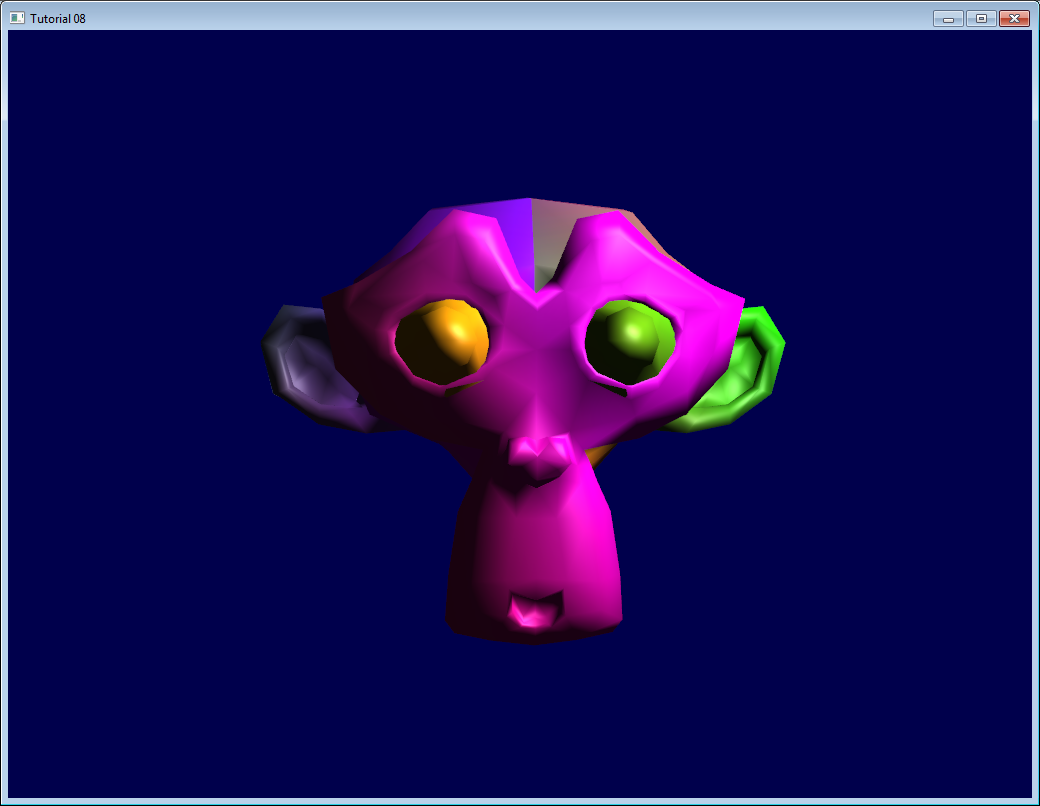
Notice the specular highlights on the nose and on the eyebrows.
This shading model has been used for years due to its simplicity. It has a number of problems, so it is replaced by physically-based models like the microfacet BRDF, but we will see this later.
In the next tutorial, we’ll learn how to improve the performance of your VBO. This will be the first Intermediate tutorial !
Tutorial 9 : VBO Indexing
- The principle of indexing
- Shared vs Separate
- Indexed VBO in OpenGL
- Filling the index buffer
- Extra : the FPS counter
The principle of indexing
Until now, when building your VBO, we always duplicated our vertices whenever two triangles shared an edge.
In this tutorial, we introduce indexing, which enables to reuse the same vertex over and over again. This is done with an index buffer.
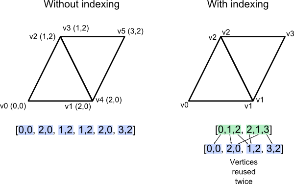
The index buffer contains integers, three for each triangle in the mesh, which reference the various attribute buffers (position, colour, UV coordinates, other UV coordinates, normal, …). It’s a little bit like in the OBJ file format, with one huge difference : there is only ONE index buffer. This means that for a vertex to be shared between two triangles, all attributes must be the same.
Shared vs Separate
Let’s take the example of the normals. In this figure, the artist who created these two triangle probably wanted them to represent a smooth surface. We can thus blend the normals of the two triangle into a single vertex normal. For visualization purposes, I added a red line which represents the aspect of the smooth surface.

In this second figure however, the artist visibly wanted a “seam”, a rough edge. But if we merge the normals, this means that the shader will smoothly interpolate as usual and create a smooth aspect just like before :
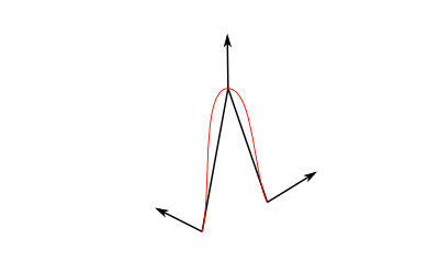
So in this case it’s actually better to have two different normals, one for each vertex. The only way to do this in OpenGL is to duplicate the whole vertex, with its whole set of attributes.
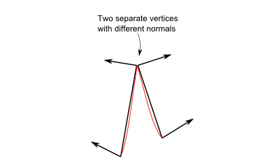
Indexed VBO in OpenGL
Using indexing is very simple. First, you need to create an additional buffer, which you fill with the right indices. The code is the same as before, but now it’s an ELEMENT_ARRAY_BUFFER, not an ARRAY_BUFFER.
std::vector<unsigned int> indices;

// fill "indices" as needed

// Generate a buffer for the indices
 GLuint elementbuffer;
 glGenBuffers(1, &elementbuffer);
 glBindBuffer(GL_ELEMENT_ARRAY_BUFFER, elementbuffer);
 glBufferData(GL_ELEMENT_ARRAY_BUFFER, indices.size() * sizeof(unsigned int), &indices[0], GL_STATIC_DRAW);
and to draw the mesh, simply replace glDrawArrays by this :
// Index buffer
 glBindBuffer(GL_ELEMENT_ARRAY_BUFFER, elementbuffer);

 // Draw the triangles !
 glDrawElements(
     GL_TRIANGLES,      // mode
     indices.size(),    // count
     GL_UNSIGNED_INT,   // type
     (void*)0           // element array buffer offset
 );
(quick note : it’s better to use “unsigned short” than “unsigned int”, because it takes less memory, which also makes it faster)
Filling the index buffer
Now we actually have a problem. As I said before, OpenGL can only use one index buffer, whereas OBJ (and some other popular 3D formats like Collada) use one index buffer by attribute. Which means that we somehow have to convert from N index buffers to 1 index buffer.
The algorithm to do this is as follows :
For each input vertex
    Try to find a similar ( = same for all attributes ) vertex between all those we already output
    If found :
        A similar vertex is already in the VBO, use it instead !
    If not found :
        No similar vertex found, add it to the VBO
The actual C++ code can be found in common/vboindexer.cpp. It’s heavily commented so if you understand the algorithm above, it should be all right.
The criterion for similarity is that vertices’ position, UVs and normals should be ** equal. You’ll have to adapt this if you add more attributes.
Searching a similar vertex is done with a lame linear search for simplicity. A std::map would be more appropriate for real use.
Extra : the FPS counter
It’s not directly related to indexing, but it’s a good moment to have a look at the FPS counter because we can eventually see the speed improvement of indexing. Other performance tools are available in Tools - Debuggers.
Tutorial 10 : Transparency
The alpha channel
The concept of the alpha channel is pretty simple. Instead of a writing an RGB result, you write an RGBA :
// Ouput data : it's now a vec4
out vec4 color;
the first 3 components are still accessed with the .xyz swizzle operator, while the last one is accessed with .a :
color.a = 0.3;
Unintuitively, alpha = opaqueness, so alpha = 1 means fully opaque while alpha = 0 means fully transparent.
Here, we simply hardcode the alpha channel at 0.3, but you probably want to use a uniform, or read it from a RGBA texture ( TGA supports the alpha channel, and GLFW supports TGA )
Here’s the result. Make sure to turn backface culling off (glDisable(GL_CULL_FACE) ) because since we can look through the mesh, we could see that it has no “back” face.
![]()
Order matters !
The previous screenshot looks okay-ish, but that’s just because we’re lucky.
The problem
Here, I drew two squares with 50% alpha, one green and one red. You can see that order is important, the final colour gives an important clue to the eyes for proper depth perception.
![]()
This phenomena also happens in our scene. Let’s change the viewpoint a bit :
![]()
It turns out that this is a very hard problem. You never see lots of transparency in games, do you ?
Usual solution
The usual solution is to sort all transparent triangles. Yes, ALL transparent triangles.
- Draw the opaque part of the world so that the depth buffer already can reject hidden transparent triangles
- Sort transparent triangles, from the furthest to the closest
- Draw the transparent triangles.
You can sort whatever you want with qsort (in C) or std::sort (in C++). I won’t dig in the details, because…
Caveat
Doing so will work ( more on this in the next section ), but :
- You will be fillrate limited. That is, each fragment will be written 10, 20 times, maybe more. This is way too much for the poor memory bus. Usually the depth buffer allows to reject enough “far” fragments, but here, you explicitly sorted them, so the depth buffer is actually useless.
- You will be doing this 4 times per pixel ( we use 4xMSAA ), except if you use some clever optimisation
- Sorting all the transparent triangles takes time
- If you have to switch your texture, or worse, your shader, from triangle to triangle, you’re going into deep performance trouble. Don’t do this.
A good enough solution is often to :
- Limit to a maximum the number of transparent polygons
- Use the same shader and the same texture for all of them
- If they are supposed to look very different, use your texture !
- If you can avoid sorting, and it still doesn’t look *too *bad, consider yourself lucky.
Order-Independent Transparency
A number of other techniques are worth investigating if your engine really, really needs state-of-the-art transparency :
- The original 2001 Depth Peeling paper: pixel-perfect results, not very fast.
- Dual Depth Peeling : a slight improvement
- Several papers on bucket sort. Uses an array of fragments; sort them by depth in a shader.
- ATI’s Mecha Demo : good and fast, but tricky to implement, needs recent hardware. Uses a linked list of fragments.
- Cyril Crassin’s variation on the ATI’s technique : even harder implementation
Note that even a recent game like Little Big Planet, which ran on a powerful console, used only 1 layer of transparency.
The blend function
In order for the previous code to work, you need to setup your blend function.
// Enable blending
glEnable(GL_BLEND);
glBlendFunc(GL_SRC_ALPHA, GL_ONE_MINUS_SRC_ALPHA);
Which means :
New color in framebuffer =
           shader's output alpha * shader's output color +
           (1 - shader's output alpha) * current color in framebuffer
Example from the image above, with red on top :
new color = 0.5*(0,1,0) + (1-0.5)*(1,0.5,0.5); // (the red was already blended with the white background)
new color = (1, 0.75, 0.25) = the same orange
Tutorial 11 : 2D text
In this tutorial, we’ll learn to draw 2D text on top of our 3D content. In our case, this will be a simple timer :
The API
We’re going to implement this simple interface (in common/text2D.h):
void initText2D(const char * texturePath);
void printText2D(const char * text, int x, int y, int size);
void cleanupText2D();
In order for the code to work at both 640*480 and 1080p, x and y will be coordinates in [0-800][0-600]. The vertex shader will adapt this to the actual size of the screen.
See common/text2D.cpp for the complete implementation.
The texture
initText2D simply reads a texture and a couple of shaders. There’s nothing fancy about it, but let’s look at the texture :
This texture was generated using CBFG, one of the many tools that generate textures from fonts. It was then imported in Paint.NET where I added a red background (for visualisation purposes only : everywhere you see red, it’s supposed to be transparent ).
The goal of printText2D will thus be to generate quads with the appropriate screen position and texture coordinates.
Drawing
We have to fill these buffers :
std::vector<glm::vec2> vertices;
std::vector<glm::vec2> UVs;
For each character, we compute the coordinates of the four vertices that will define the quad, and add the two triangles :
for ( unsigned int i=0 ; i<length ; i++ ){

    glm::vec2 vertex_up_left    = glm::vec2( x+i*size     , y+size );
    glm::vec2 vertex_up_right   = glm::vec2( x+i*size+size, y+size );
    glm::vec2 vertex_down_right = glm::vec2( x+i*size+size, y      );
    glm::vec2 vertex_down_left  = glm::vec2( x+i*size     , y      );

    vertices.push_back(vertex_up_left   );
    vertices.push_back(vertex_down_left );
    vertices.push_back(vertex_up_right  );

    vertices.push_back(vertex_down_right);
    vertices.push_back(vertex_up_right);
    vertices.push_back(vertex_down_left);
Now for the UVs. The upper-left coordinate is computed as follows :
    char character = text[i];
    float uv_x = (character%16)/16.0f;
    float uv_y = (character/16)/16.0f;
This works ( sort of - see below ) because the ASCII code for A is 65.
65%16 = 1, so A is on column #1 (starts at 0 !).
65/16 = 4, so A is on line #4 ( it’s integer division, so it’s not 4.0625 as it should be)
Both are divided by 16.0 to fit in the [0.0 - 1.0] range needed by OpenGL textures.
And now we just have to do the very same thing than we did, but for the vertices :
    glm::vec2 uv_up_left    = glm::vec2( uv_x           , 1.0f - uv_y );
    glm::vec2 uv_up_right   = glm::vec2( uv_x+1.0f/16.0f, 1.0f - uv_y );
    glm::vec2 uv_down_right = glm::vec2( uv_x+1.0f/16.0f, 1.0f - (uv_y + 1.0f/16.0f) );
    glm::vec2 uv_down_left  = glm::vec2( uv_x           , 1.0f - (uv_y + 1.0f/16.0f) );

    UVs.push_back(uv_up_left   );
    UVs.push_back(uv_down_left );
    UVs.push_back(uv_up_right  );

    UVs.push_back(uv_down_right);
    UVs.push_back(uv_up_right);
    UVs.push_back(uv_down_left);
 }
The rest is just as usual : bind the buffers, fill them, select the shader program, bind the texture, enable/bind/configure the vertex attributes, enable the blending, and call glDrawArrays. Hooray ! You’re done.
Note a very important thing : the coordinates are generated in the [0,800][0,600] range. In other words, there is NO NEED for a matrix here. The vertex shader simply has to put it in the [-1,1][-1,1] range with very simple math (this could be done in C++ too) :
void main(){

    // Output position of the vertex, in clip space
    // map [0..800][0..600] to [-1..1][-1..1]
    vec2 vertexPosition_homoneneousspace = vertexPosition_screenspace - vec2(400,300); // [0..800][0..600] -> [-400..400][-300..300]
    vertexPosition_homoneneousspace /= vec2(400,300);
    gl_Position =  vec4(vertexPosition_homoneneousspace,0,1);

    // UV of the vertex. No special space for this one.
    UV = vertexUV;
}
The fragment shader does very little too :
void main(){
    color = texture( myTextureSampler, UV );
}
By the way, don’t use this code for production, since it only handles the Latin alphabet. Or don’t sell anything to India, China, Japan ( or even Germany, since there is no ß on this image ). This texture will mostly work in France (notice the é, à, ç, etc) because it’s been generated with my locale. And beware while adapting code from other tutorials of when using libraries, most of them use OpenGL 2, which isn’t compatible. Unfortunately I don’t know any good-enough library which handles UTF-8.
By the way, you should read The Absolute Minimum Every Software Developer Absolutely, Positively Must Know About Unicode and Character Sets (No Excuses!) by Joel Spolsky.
See also this Valve article if you need large text.
Tutorial 12 : OpenGL Extensions
Extensions
With each new generation, the performance of GPU increases, allowing to render more triangles and more pixels. However, raw performance isn’t the only concern. NVIDIA, AMD and Intel also improve their graphic cards by providing more functionality. Let’s have a look at some examples.
ARB_fragment_program
Back in 2002, GPUs had no vertex shaders or fragment shaders : everything was hardcoded inside the chip. This was called the Fixed-Function Pipeline (FFP). As such, the most recent version of the API, which was OpenGL 1.3, proposed no way to create, manipulate and use so-called “shaders”, since it didn’t even exist. But then NVIDIA decided that it could be handy to describe the rendering process with actual code, instead of hundreds of flags and state variables. This is how ARB_fragment_program was created : there was no GLSL, but instead you could write stuff like this :
!!ARBfp1.0 MOV result.color, fragment.color; END
But obviously to tell OpenGL to use such code, you needed special functions, which were not yet in OpenGL. Before moving on to the explanations, one more example.
ARB_debug_output
Ok, you say, but this ARB_fragment_program is too old, surely I don’t need this extension stuff anymore ? Well there are newer extensions which are very handy. One of them is ARB_debug_output, which expose a functionality that doesn’t exist in OpenGL 3.3 but that you can/should use anyway. It defines tokens like GL_DEBUG_OUTPUT_SYNCHRONOUS_ARB or GL_DEBUG_SEVERITY_MEDIUM_ARB, and functions like DebugMessageCallbackARB. The great thing about this extension is that whenever you write some incorrect code, for instance :
glEnable(GL_TEXTURE); // Incorrect ! You probably meant GL_TEXTURE_2D !
you can have an error message and the exact location of the problem. Lessons learned :
- Extensions are still very useful, even in modern, 3.3 OpenGL
- Use ARB_debug_output ! See below for links.
Getting an extension - the hard way
The “manual” way for checking is an extension is present is to use this code snippet (from the OpenGL.org wiki) :
int NumberOfExtensions;
glGetIntegerv(GL_NUM_EXTENSIONS, &NumberOfExtensions);
for(i=0; i<NumberOfExtensions; i++) {
  const GLubyte *ccc=glGetStringi(GL_EXTENSIONS, i);
  if ( strcmp(ccc, (const GLubyte *)"GL_ARB_debug_output") == 0 ){
    // The extension is supported by our hardware and driver
    // Try to get the "glDebugMessageCallbackARB" function :
    glDebugMessageCallbackARB  = (PFNGLDEBUGMESSAGECALLBACKARBPROC) wglGetProcAddress("glDebugMessageCallbackARB");
  }
}
Getting all extensions - the easy way
All in all this is very complicated. Libraries like GLEW, GLee, gl3w, etc, make it much easier. For instance, with GLEW, you just have to call glewInit() after you created your window, and handy variables are created :
if (GLEW_ARB_debug_output){ // Ta-Dah ! }
( a word of caution : debug_output is special because you have to enable it at context creation. In GLFW, this is done with glfwOpenWindowHint(GLFW_OPENGL_DEBUG_CONTEXT, 1); )
ARB vs EXT vs …
The name of each extention contains information on its availability :
GL_ : all platforms; GLX_ : Linux & Mac only (X11); WGL_ : Windows only
EXT : A generic extention. ARB : the extention has been accepted by all the members of the OpenGL Architecture Review Board (EXT extentions are often promoted to ARB after a while). NV/AMD/INTEL : Quite self-explanatory =)
Designing with Extentions
The problem
Let’s say that your OpenGL 3.3 application needs to render some large lines. You could write a complicated vertex shader to do that, or simply rely on GL_NV_path_rendering, which will handle all the complicated stuff for you.
You will thus have code that look like this :
if ( GLEW_NV_path_rendering ){
    glPathStringNV( ... ); // Draw the shape. Easy !
}else{
    // Else what ? You still have to draw the lines
    // on older NVIDIA hardware, on AMD and on INTEL !
    // So you have to implement it yourself anyway !
}
Choosing the limit
One usually choose to use an extention when the gain in rendering quality or performance outweights the pain of maintaining two different paths.
For instance, Braid (the 2D game where you travel in time) has all kinds of image-warping effects when you mess with the time, which simply aren’t rendered on older hardware.
With OpenGL 3.3 and above, you already have 99% of the tools you’re likely to need. Some extensions can be very useful, like GL_AMD_pinned_memory, but this is often not like a few years ago when having GL_ARB_framebuffer_object ( used for Render To Texture ) could make your game look 10 times better.
If you have to handle older hardware, though, OpenGL 3+ won’t be available, and you’ll have to use OpenGL 2+ instead. You won’t be able to assume that you have all the fancy extensions anymore, and you’ll need to cope with that.
For further details, see for instance the OpenGL 2.1 version of Tutorial 14 - Render To Texture, line 167, where I have to check the presence of GL_ARB_framebuffer_object by hand. See also the FAQ.
Conclusion
OpenGL Extentions provide a nice way to extend OpenGL’s capabilities, depending on your user’s GPU.
While extentions are nowaday mostly for advanced use since most functionality is already in the core, it’s still important to know how they work and how you can use them to improve your software - at the expense of higher maintainance.
Further reading
- debug_output tutorial by Aks you can skip Step 1 thanks to GLEW.
- The OpenGL extension registry All extensions specifications. The bible.
- GLEW The OpenGL Extension Wrangler Library
- gl3w Simple OpenGL 3/4 core profile loading
Tutorial 13 : Normal Mapping
- Normal textures
- Tangent and Bitangent
- Preparing our VBO
- The shader
- Results
- Going further
- Exercises
- Tools & Links
- References
Welcome for our 13th tutorial ! Today we will talk about normal mapping.
Since Tutorial 8 : Basic shading, you know how to get decent shading using triangle normals. One caveat is that until now, we only had one normal per vertex : inside each triangle, they vary smoothly, on the opposite to the colour, which samples a texture. The basic idea of normal mapping is to give normals similar variations.
Normal textures
A “normal texture” looks like this :
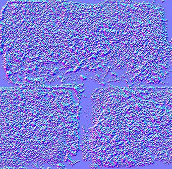
In each RGB texel is encoded a XYZ vector : each colour component is between 0 and 1, and each vector component is between -1 and 1, so this simple mapping goes from the texel to the normal :
normal = (2*color)-1 // on each component
The texture has a general blue tone because overall, the normal is towards the “outside of the surface”. As usual, X is right in the plane of the texture, Y is up (again in the plane of the texture), thus given the right hand rule Z point to the “outside” of the plane of the texture.
This texture is mapped just like the diffuse one; the big problem is how to convert our normal, which is expressed in the space each individual triangle (tangent space, also called image space), in model space (since this is what is used in our shading equation).
Tangent and Bitangent
You are now so familiar with matrices that you know that in order to define a space (in our case, the tangent space), we need 3 vectors. We already have our UP vector : it’s the normal, given by Blender or computed from the triangle by a simple cross product. It’s represented in blue, just like the overall color of the normal map :

Next we need a tangent, T : a vector parallel to the surface. But there are many such vectors :

Which one should we choose ? In theory, any, but we have to be consistent with the neighbors to avoid introducing ugly edges. The standard method is to orient the tangent in the same direction that our texture coordinates :

Since we need 3 vectors to define a basis, we must also compute the bitangent B (which is any other tangent vector, but if everything is perpendicular, math is simpler) :

Here is the algorithm : if we note deltaPos1 and deltaPos2 two edges of our triangle, and deltaUV1 and deltaUV2 the corresponding differences in UVs, we can express our problem with the following equation :
deltaPos1 = deltaUV1.x * T + deltaUV1.y * B
deltaPos2 = deltaUV2.x * T + deltaUV2.y * B
Just solve this system for T and B, and you have your vectors ! (See code below)
Once we have our T, B, N vectors, we also have this nice matrix which enables us to go from Tangent Space to Model Space :
With this TBN matrix, we can transform normals (extracted from the texture) into model space. However, it’s usually done the other way around : transform everything from Model Space to Tangent Space, and keep the extracted normal as-is. All computations are done in Tangent Space, which doesn’t changes anything.
Do have this inverse transformation, we simply have to take the matrix inverse, which in this case (an orthogonal matrix, i.e each vector is perpendicular to the others. See “going further” below) is also its transpose, much cheaper to compute :
invTBN = transpose(TBN)
, i.e. :
![]()
Preparing our VBO
Computing the tangents and bitangents
Since we need our tangents and bitangents on top of our normals, we have to compute them for the whole mesh. We’ll do this in a separate function :
void computeTangentBasis(
    // inputs
    std::vector<glm::vec3> & vertices,
    std::vector<glm::vec2> & uvs,
    std::vector<glm::vec3> & normals,
    // outputs
    std::vector<glm::vec3> & tangents,
    std::vector<glm::vec3> & bitangents
){
For each triangle, we compute the edge (deltaPos) and the deltaUV
    for ( int i=0; i<vertices.size(); i+=3){

        // Shortcuts for vertices
        glm::vec3 & v0 = vertices[i+0];
        glm::vec3 & v1 = vertices[i+1];
        glm::vec3 & v2 = vertices[i+2];

        // Shortcuts for UVs
        glm::vec2 & uv0 = uvs[i+0];
        glm::vec2 & uv1 = uvs[i+1];
        glm::vec2 & uv2 = uvs[i+2];

        // Edges of the triangle : position delta
        glm::vec3 deltaPos1 = v1-v0;
        glm::vec3 deltaPos2 = v2-v0;

        // UV delta
        glm::vec2 deltaUV1 = uv1-uv0;
        glm::vec2 deltaUV2 = uv2-uv0;
We can now use our formula to compute the tangent and the bitangent :
        float r = 1.0f / (deltaUV1.x * deltaUV2.y - deltaUV1.y * deltaUV2.x);
        glm::vec3 tangent = (deltaPos1 * deltaUV2.y   - deltaPos2 * deltaUV1.y)*r;
        glm::vec3 bitangent = (deltaPos2 * deltaUV1.x   - deltaPos1 * deltaUV2.x)*r;
Finally, we fill the *tangents *and *bitangents *buffers. Remember, these buffers are not indexed yet, so each vertex has its own copy.
        // Set the same tangent for all three vertices of the triangle.
        // They will be merged later, in vboindexer.cpp
        tangents.push_back(tangent);
        tangents.push_back(tangent);
        tangents.push_back(tangent);

        // Same thing for bitangents
        bitangents.push_back(bitangent);
        bitangents.push_back(bitangent);
        bitangents.push_back(bitangent);

    }
Indexing
Indexing our VBO is very similar to what we used to do, but there is a subtle difference.
If we find a similar vertex (same position, same normal, same texture coordinates), we don’t want to use its tangent and bitangent too ; on the contrary, we want to average them. So let’s modify our old code a bit :
        // Try to find a similar vertex in out_XXXX
        unsigned int index;
        bool found = getSimilarVertexIndex(in_vertices[i], in_uvs[i], in_normals[i],     out_vertices, out_uvs, out_normals, index);

        if ( found ){ // A similar vertex is already in the VBO, use it instead !
            out_indices.push_back( index );

            // Average the tangents and the bitangents
            out_tangents[index] += in_tangents[i];
            out_bitangents[index] += in_bitangents[i];
        }else{ // If not, it needs to be added in the output data.
            // Do as usual
            [...]
        }
Note that we don’t normalize anything here. This is actually handy, because this way, small triangles, which have smaller tangent and bitangent vectors, will have a weaker effect on the final vectors than big triangles (which contribute more to the final shape).
The shader
Additional buffers & uniforms
We need two new buffers : one for the tangents, and one for the bitangents :
    GLuint tangentbuffer;
    glGenBuffers(1, &tangentbuffer);
    glBindBuffer(GL_ARRAY_BUFFER, tangentbuffer);
    glBufferData(GL_ARRAY_BUFFER, indexed_tangents.size() * sizeof(glm::vec3), &indexed_tangents[0], GL_STATIC_DRAW);

    GLuint bitangentbuffer;
    glGenBuffers(1, &bitangentbuffer);
    glBindBuffer(GL_ARRAY_BUFFER, bitangentbuffer);
    glBufferData(GL_ARRAY_BUFFER, indexed_bitangents.size() * sizeof(glm::vec3), &indexed_bitangents[0], GL_STATIC_DRAW);
We also need a new uniform for our new normal texture :
    [...]
    GLuint NormalTexture = loadTGA_glfw("normal.tga");
    [...]
    GLuint NormalTextureID  = glGetUniformLocation(programID, "NormalTextureSampler");
And one for the 3x3 ModelView matrix. This is strictly speaking not necessary, but it’s easier ; more about this later. We just need the 3x3 upper-left part because we will multiply directions, so we can drop the translation part.
GLuint ModelView3x3MatrixID = glGetUniformLocation(programID, "MV3x3");
So the full drawing code becomes :
        // Clear the screen
        glClear(GL_COLOR_BUFFER_BIT | GL_DEPTH_BUFFER_BIT);

        // Use our shader
        glUseProgram(programID);

        // Compute the MVP matrix from keyboard and mouse input
        computeMatricesFromInputs();
        glm::mat4 ProjectionMatrix = getProjectionMatrix();
        glm::mat4 ViewMatrix = getViewMatrix();
        glm::mat4 ModelMatrix = glm::mat4(1.0);
        glm::mat4 ModelViewMatrix = ViewMatrix * ModelMatrix;
        glm::mat3 ModelView3x3Matrix = glm::mat3(ModelViewMatrix); // Take the upper-left part of ModelViewMatrix
        glm::mat4 MVP = ProjectionMatrix * ViewMatrix * ModelMatrix;

        // Send our transformation to the currently bound shader,
        // in the "MVP" uniform
        glUniformMatrix4fv(MatrixID, 1, GL_FALSE, &MVP[0][0]);
        glUniformMatrix4fv(ModelMatrixID, 1, GL_FALSE, &ModelMatrix[0][0]);
        glUniformMatrix4fv(ViewMatrixID, 1, GL_FALSE, &ViewMatrix[0][0]);
        glUniformMatrix4fv(ViewMatrixID, 1, GL_FALSE, &ViewMatrix[0][0]);
        glUniformMatrix3fv(ModelView3x3MatrixID, 1, GL_FALSE, &ModelView3x3Matrix[0][0]);

        glm::vec3 lightPos = glm::vec3(0,0,4);
        glUniform3f(LightID, lightPos.x, lightPos.y, lightPos.z);

        // Bind our diffuse texture in Texture Unit 0
        glActiveTexture(GL_TEXTURE0);
        glBindTexture(GL_TEXTURE_2D, DiffuseTexture);
        // Set our "DiffuseTextureSampler" sampler to user Texture Unit 0
        glUniform1i(DiffuseTextureID, 0);

        // Bind our normal texture in Texture Unit 1
        glActiveTexture(GL_TEXTURE1);
        glBindTexture(GL_TEXTURE_2D, NormalTexture);
        // Set our "Normal    TextureSampler" sampler to user Texture Unit 0
        glUniform1i(NormalTextureID, 1);

        // 1rst attribute buffer : vertices
        glEnableVertexAttribArray(0);
        glBindBuffer(GL_ARRAY_BUFFER, vertexbuffer);
        glVertexAttribPointer(
            0,                  // attribute
            3,                  // size
            GL_FLOAT,           // type
            GL_FALSE,           // normalized?
            0,                  // stride
            (void*)0            // array buffer offset
        );

        // 2nd attribute buffer : UVs
        glEnableVertexAttribArray(1);
        glBindBuffer(GL_ARRAY_BUFFER, uvbuffer);
        glVertexAttribPointer(
            1,                                // attribute
            2,                                // size
            GL_FLOAT,                         // type
            GL_FALSE,                         // normalized?
            0,                                // stride
            (void*)0                          // array buffer offset
        );

        // 3rd attribute buffer : normals
        glEnableVertexAttribArray(2);
        glBindBuffer(GL_ARRAY_BUFFER, normalbuffer);
        glVertexAttribPointer(
            2,                                // attribute
            3,                                // size
            GL_FLOAT,                         // type
            GL_FALSE,                         // normalized?
            0,                                // stride
            (void*)0                          // array buffer offset
        );

        // 4th attribute buffer : tangents
        glEnableVertexAttribArray(3);
        glBindBuffer(GL_ARRAY_BUFFER, tangentbuffer);
        glVertexAttribPointer(
            3,                                // attribute
            3,                                // size
            GL_FLOAT,                         // type
            GL_FALSE,                         // normalized?
            0,                                // stride
            (void*)0                          // array buffer offset
        );

        // 5th attribute buffer : bitangents
        glEnableVertexAttribArray(4);
        glBindBuffer(GL_ARRAY_BUFFER, bitangentbuffer);
        glVertexAttribPointer(
            4,                                // attribute
            3,                                // size
            GL_FLOAT,                         // type
            GL_FALSE,                         // normalized?
            0,                                // stride
            (void*)0                          // array buffer offset
        );

        // Index buffer
        glBindBuffer(GL_ELEMENT_ARRAY_BUFFER, elementbuffer);

        // Draw the triangles !
        glDrawElements(
            GL_TRIANGLES,      // mode
            indices.size(),    // count
            GL_UNSIGNED_INT,   // type
            (void*)0           // element array buffer offset
        );

        glDisableVertexAttribArray(0);
        glDisableVertexAttribArray(1);
        glDisableVertexAttribArray(2);
        glDisableVertexAttribArray(3);
        glDisableVertexAttribArray(4);

        // Swap buffers
        glfwSwapBuffers();
Vertex shader
As said before, we’ll do everything in camera space, because it’s simpler to get the fragment’s position in this space. This is why we multiply our T,B,N vectors with the ModelView matrix.
    vertexNormal_cameraspace = MV3x3 * normalize(vertexNormal_modelspace);
    vertexTangent_cameraspace = MV3x3 * normalize(vertexTangent_modelspace);
    vertexBitangent_cameraspace = MV3x3 * normalize(vertexBitangent_modelspace);
These three vector define the TBN matrix, which is constructed this way :
    mat3 TBN = transpose(mat3(
        vertexTangent_cameraspace,
        vertexBitangent_cameraspace,
        vertexNormal_cameraspace
    )); // You can use dot products instead of building this matrix and transposing it. See References for details.
This matrix goes from camera space to tangent space (The same matrix, but with XXX_modelspace instead, would go from model space to tangent space). We can use it to compute the light direction and the eye direction, in tangent space :
    LightDirection_tangentspace = TBN * LightDirection_cameraspace;
    EyeDirection_tangentspace =  TBN * EyeDirection_cameraspace;
Fragment shader
Our normal, in tangent space, is really straightforward to get : it’s our texture :
    // Local normal, in tangent space
    vec3 TextureNormal_tangentspace = normalize(texture( NormalTextureSampler, UV ).rgb*2.0 - 1.0);
So we’ve got everything we need now. Diffuse lighting uses clamp( dot( n,l ), 0,1 ), with n and l expressed in tangent space (it doesn’t matter in which space you make your dot and cross products; the important thing is that n and l are both expressed in the same space). Specular lighting uses clamp( dot( E,R ), 0,1 ), again with E and R expressed in tangent space. Yay !
Results
Here is our result so far. You can notice that :
- The bricks look bumpy because we have lots of variations in the normals
- Cement looks flat because the normal texture is uniformly blue
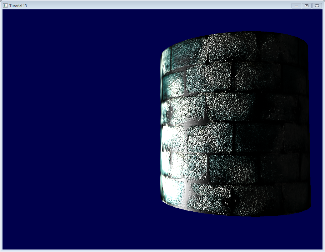
Going further
Orthogonalization
In our vertex shader we took the transpose instead of the inverse because it’s faster. But it only works if the space that the matrix represents is orthogonal, which is not yet the case. Luckily, this is very easy to fix : we just have to make the tangent perpendicular to the normal at he end of computeTangentBasis() :
t = glm::normalize(t - n * glm::dot(n, t));
This formula may be hard to grasp, so a little schema might help :

n and t are almost perpendicular, so we “push” t in the direction of -n by a factor of dot(n,t)
Here’s a little applet that explains it too (Use only 2 vectors).
Handedness
You usually don’t have to worry about that, but in some cases, when you use symmetric models, UVs are oriented in the wrong way, and your T has the wrong orientation.
To check whether it must be inverted or not, the check is simple : TBN must form a right-handed coordinate system, i.e. cross(n,t) must have the same orientation than b.
In mathematics, “Vector A has the same orientation as Vector B” translates as dot(A,B)>0, so we need to check if dot( cross(n,t) , b ) > 0.
If it’s false, just invert t :
if (glm::dot(glm::cross(n, t), b) < 0.0f){
     t = t * -1.0f;
 }
This is also done for each vertex at the end of computeTangentBasis().
Specular texture
Just for fun, I added a specular texture to the code. It looks like this :

and is used instead of the simple “vec3(0.3,0.3,0.3)” grey that we used as specular color.
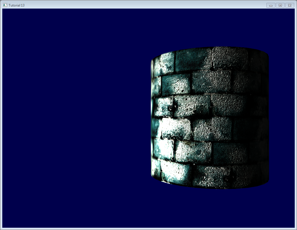
Notice that now, cement is always black : the texture says that it has no specular component.
Debugging with the immediate mode
The real aim of this website is that you DON’T use immediate mode, which is deprecated, slow, and problematic in many aspects.
However, it also happens to be really handy for debugging :

Here we visualize our tangent space with lines drawn in immediate mode.
For this, you need to abandon the 3.3 core profile :
glfwOpenWindowHint(GLFW_OPENGL_PROFILE, GLFW_OPENGL_COMPAT_PROFILE);
then give our matrices to OpenGL’s old-school pipeline (you can write another shader too, but it’s simpler this way, and you’re hacking anyway) :
glMatrixMode(GL_PROJECTION);
glLoadMatrixf((const GLfloat*)&ProjectionMatrix[0]);
glMatrixMode(GL_MODELVIEW);
glm::mat4 MV = ViewMatrix * ModelMatrix;
glLoadMatrixf((const GLfloat*)&MV[0]);
Disable shaders :
glUseProgram(0);
And draw your lines (in this case, normals, normalized and multiplied by 0.1, and applied at the correct vertex) :
glColor3f(0,0,1);
glBegin(GL_LINES);
for (int i=0; i<indices.size(); i++){
    glm::vec3 p = indexed_vertices[indices[i]];
    glVertex3fv(&p.x);
    glm::vec3 o = glm::normalize(indexed_normals[indices[i]]);
    p+=o*0.1f;
    glVertex3fv(&p.x);
}
glEnd();
Remember : don’t use immediate mode in real world ! Only for debugging ! And don’t forget to re-enable the core profile afterwards, it will make sure that you don’t do such things.
Debugging with colors
When debugging, it can be useful to visualize the value of a vector. The easiest way to do this is to write it on the framebuffer instead of the actual colour. For instance, let’s visualize LightDirection_tangentspace :
color.xyz = LightDirection_tangentspace;

This means :
- On the right part of the cylinder, the light (represented by the small white line) is UP (in tangent space). In other words, the light is in the direction of the normal of the triangles.
- On the middle part of the cylinder, the light is in the direction of the tangent (towards +X)
A few tips :
- Depending on what you’re trying to visualize, you may want to normalize it.
- If you can’t make sense of what you’re seeing, visualize all components separately by forcing for instance green and blue to 0.
- Avoid messing with alpha, it’s too complicated :)
- If you want to visualize negative value, you can use the same trick that our normal textures use : visualize (v+1.0)/2.0 instead, so that black means -1 and full color means +1. It’s hard to understand what you see, though.
Debugging with variable names
As already stated before, it’s crucial to exactly know in which space your vectors are. Don’t take the dot product of a vector in camera space and a vector in model space.
Appending the space of each vector in their names (“…_modelspace”) helps fixing math bugs tremendously.
How to create a normal map
Created by James O’Hare. Click to enlarge.
Exercises
- Normalize the vectors in indexVBO_TBN before the addition and see what it does.
- Visualize other vectors (for instance, EyeDirection_tangentspace) in color mode, and try to make sense of what you see
Tools & Links
- Crazybump , a great tool to make normal maps. Not free.
- Nvidia’s photoshop plugin. Free, but photoshop isn’t…
- Make your own normal maps out of several photos
- Make your own normal maps out of one photo
- Some more info on matrix transpose
References
Tutorial 14 : Render To Texture
Render-To-Texture is a handful method to create a variety of effects. The basic idea is that you render a scene just like you usually do, but this time in a texture that you can reuse later.
Applications include in-game cameras, post-processing, and as many GFX as you can imagine.
Render To Texture
We have three tasks : creating the texture in which we’re going to render ; actually rendering something in it ; and using the generated texture.
Creating the Render Target
What we’re going to render to is called a Framebuffer. It’s a container for textures and an optional depth buffer. It’s created just like any other object in OpenGL :
// The framebuffer, which regroups 0, 1, or more textures, and 0 or 1 depth buffer.
GLuint FramebufferName = 0;
glGenFramebuffers(1, &FramebufferName);
glBindFramebuffer(GL_FRAMEBUFFER, FramebufferName);
Now we need to create the texture which will contain the RGB output of our shader. This code is very classic :
// The texture we're going to render to
GLuint renderedTexture;
glGenTextures(1, &renderedTexture);

// "Bind" the newly created texture : all future texture functions will modify this texture
glBindTexture(GL_TEXTURE_2D, renderedTexture);

// Give an empty image to OpenGL ( the last "0" )
glTexImage2D(GL_TEXTURE_2D, 0,GL_RGB, 1024, 768, 0,GL_RGB, GL_UNSIGNED_BYTE, 0);

// Poor filtering. Needed !
glTexParameteri(GL_TEXTURE_2D, GL_TEXTURE_MAG_FILTER, GL_NEAREST);
glTexParameteri(GL_TEXTURE_2D, GL_TEXTURE_MIN_FILTER, GL_NEAREST);
We also need a depth buffer. This is optional, depending on what you actually need to draw in your texture; but since we’re going to render Suzanne, we need depth-testing.
// The depth buffer
GLuint depthrenderbuffer;
glGenRenderbuffers(1, &depthrenderbuffer);
glBindRenderbuffer(GL_RENDERBUFFER, depthrenderbuffer);
glRenderbufferStorage(GL_RENDERBUFFER, GL_DEPTH_COMPONENT, 1024, 768);
glFramebufferRenderbuffer(GL_FRAMEBUFFER, GL_DEPTH_ATTACHMENT, GL_RENDERBUFFER, depthrenderbuffer);
Finally, we configure our framebuffer
// Set "renderedTexture" as our colour attachement #0
glFramebufferTexture(GL_FRAMEBUFFER, GL_COLOR_ATTACHMENT0, renderedTexture, 0);

// Set the list of draw buffers.
GLenum DrawBuffers[1] = {GL_COLOR_ATTACHMENT0};
glDrawBuffers(1, DrawBuffers); // "1" is the size of DrawBuffers
Something may have gone wrong during the process, depending on the capabilities of the GPU. This is how you check it :
// Always check that our framebuffer is ok
if(glCheckFramebufferStatus(GL_FRAMEBUFFER) != GL_FRAMEBUFFER_COMPLETE)
return false;
Rendering to the texture
Rendering to the texture is straightforward. Simply bind your framebuffer, and draw your scene as usual. Easy !
// Render to our framebuffer
glBindFramebuffer(GL_FRAMEBUFFER, FramebufferName);
glViewport(0,0,1024,768); // Render on the whole framebuffer, complete from the lower left corner to the upper right
The fragment shader just needs a minor adaptation :
layout(location = 0) out vec3 color;
This means that when writing in the variable “color”, we will actually write in the Render Target 0, which happens to be our texture because DrawBuffers[0] is GL_COLOR_ATTACHMENTi, which is, in our case, renderedTexture.
To recap :
- color will be written to the first buffer because of layout(location=0).
- The first buffer is GL_COLOR_ATTACHMENT0 because of DrawBuffers[1] = {GL_COLOR_ATTACHMENT0}
- GL_COLOR_ATTACHMENT0 has renderedTexture attached, so this is where your color is written.
- In other words, you can replace GL_COLOR_ATTACHMENT0 by GL_COLOR_ATTACHMENT2 and it will still work.
Note : there is no layout(location=i) in OpenGL < 3.3, but you use glFragData[i] = mvvalue anyway.
Using the rendered texture
We’re going to draw a simple quad that fills the screen. We need the usual buffers, shaders, IDs, …
// The fullscreen quad's FBO
GLuint quad_VertexArrayID;
glGenVertexArrays(1, &quad_VertexArrayID);
glBindVertexArray(quad_VertexArrayID);

static const GLfloat g_quad_vertex_buffer_data[] = {
    -1.0f, -1.0f, 0.0f,
    1.0f, -1.0f, 0.0f,
    -1.0f,  1.0f, 0.0f,
    -1.0f,  1.0f, 0.0f,
    1.0f, -1.0f, 0.0f,
    1.0f,  1.0f, 0.0f,
};

GLuint quad_vertexbuffer;
glGenBuffers(1, &quad_vertexbuffer);
glBindBuffer(GL_ARRAY_BUFFER, quad_vertexbuffer);
glBufferData(GL_ARRAY_BUFFER, sizeof(g_quad_vertex_buffer_data), g_quad_vertex_buffer_data, GL_STATIC_DRAW);

// Create and compile our GLSL program from the shaders
GLuint quad_programID = LoadShaders( "Passthrough.vertexshader", "SimpleTexture.fragmentshader" );
GLuint texID = glGetUniformLocation(quad_programID, "renderedTexture");
GLuint timeID = glGetUniformLocation(quad_programID, "time");
Now you want to render to the screen. This is done by using 0 as the second parameter of glBindFramebuffer.
// Render to the screen
glBindFramebuffer(GL_FRAMEBUFFER, 0);
glViewport(0,0,1024,768); // Render on the whole framebuffer, complete from the lower left corner to the upper right
We can draw our full-screen quad with such a shader:
#version 330 core

in vec2 UV;

out vec3 color;

uniform sampler2D renderedTexture;
uniform float time;

void main(){
    color = texture( renderedTexture, UV + 0.005*vec2( sin(time+1024.0*UV.x),cos(time+768.0*UV.y)) ).xyz;
}
This code simply sample the texture, but adds a tiny offset which depends on time.
Results
Going further
Using the depth
In some cases you might need the depth when using the rendered texture. In this case, simply render to a texture created as follows :
glTexImage2D(GL_TEXTURE_2D, 0,GL_DEPTH_COMPONENT24, 1024, 768, 0,GL_DEPTH_COMPONENT, GL_FLOAT, 0);
(“24” is the precision, in bits. You can choose between 16, 24 and 32, depending on your needs. Usually 24 is fine)
This should be enough to get you started, but the provided source code implements this too.
Note that this should be somewhat slower, because the driver won’t be able to use some optimisations such as Hi-Z.
In this screenshot, the depth levels are artificially “prettified”. Usually, its much more difficult to see anything on a depth texture. Near = Z near 0 = black, far = Z near 1 = white.
Multisampling
You can write to multisampled textures instead of “basic” textures : you just have to replace glTexImage2D by glTexImage2DMultisample in the C++ code, and sampler2D/texture by sampler2DMS/texelFetch in the fragment shader.
There is a big caveat, though : texelFetch needs another argument, which is the number of the sample to fetch. In other words, there is no automatic “filtering” (the correct term, when talking about multisampling, is “resolution”).
So you may have to resolve the MS texture yourself, in another, non-MS texture, thanks to yet another shader.
Nothing difficult, but it’s just bulky.
Multiple Render Targets
You may write to several textures at the same time.
Simply create several textures (all with the correct and same size !), call glFramebufferTexture with a different color attachement for each, call glDrawBuffers with updated parameters ( something like (2,{GL_COLOR_ATTACHMENT0,GL_COLOR_ATTACHMENT1}})), and add another output variable in your fragment shader :
layout(location = 1) out vec3 normal_tangentspace; // or whatever
Hint : If you effectively need to output a vector in a texture, floating-point textures exist, with 16 or 32 bit precision instead of 8… See glTexImage2D’s reference (search for GL_FLOAT).
Hint2 : For previous versions of OpenGL, use glFragData[1] = myvalue instead.
Exercices
- Try using glViewport(0,0,512,768); instead of glViewport(0,0,1024,768); (try with both the framebuffer and the screen)
- Experiment with other UV coordinates in the last fragment shader
- Transform the quad with a real transformation matrix. First hardcode it, and then try to use the functions of controls.hpp ; what do you notice ?
Tutorial 15 : Lightmaps
Introduction
This a video-only tutorial. It doesn’t introduce any new OpenGL-specific technique/syntax, but shows you how to use the techniques you already know to build high-quality shadows.
This tutorials explains how to build a simple world in Blender, and bake the lightmaps so that you can use them in your application.
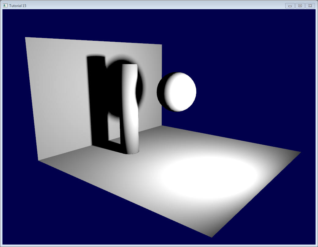
No prior knowledge of Blender is required. I will explain all keyboard shortcuts and everything.
A note on lightmaps
Lightmaps are baked. Once and for all. This means that they are completely static, you can’t decide to move the light at runtime. Or even remove it.
This can still be useful for the sunlight, though, or indoor scenes where you may not break the light bulbs. Mirror Edge, released in 2009, uses them extensively, both indoors and outdoors.
What’s more, it’s very easy to setup, and you can’t beat the speed.
The video
This is a 1024x768p video, use HD mode…
Addendum
When rendering it in OpenGL, you might notice some glitches (exaggerated here) :
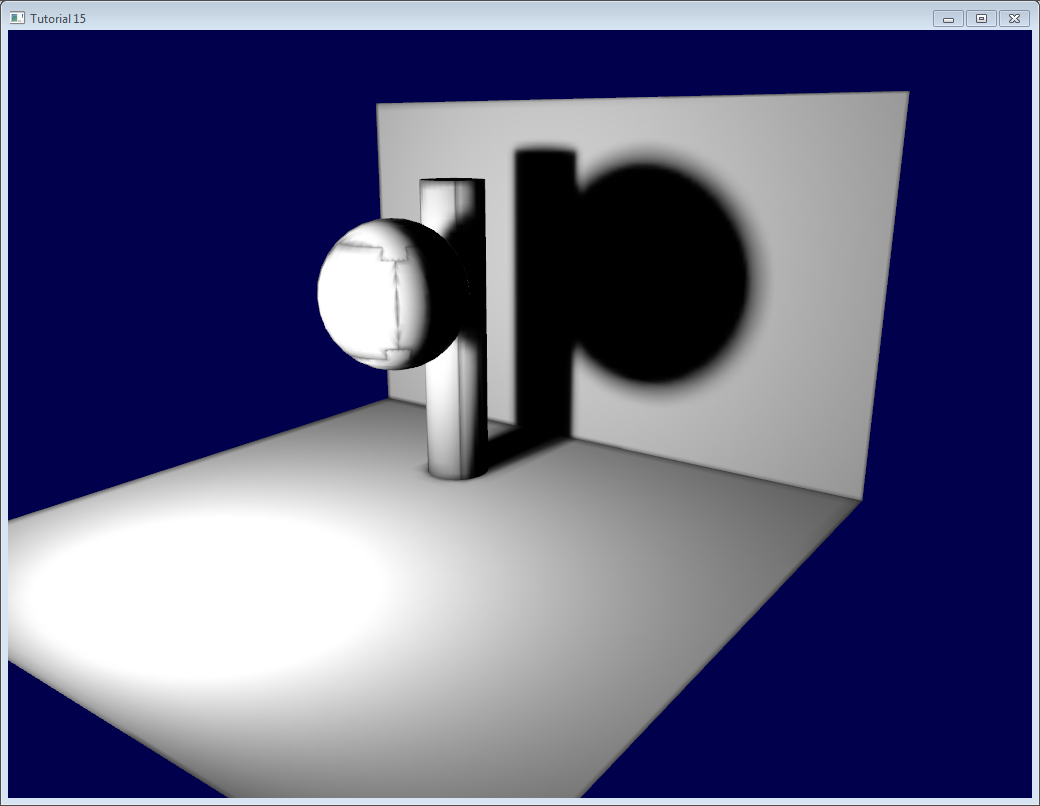
This is because of mipmapping, which blends texels together when seen at a distance. Black pixels from the texture’s background get mixed with good parts of the lightmap. To avoid this, there are a few things you can do :
- You can ask Blender to generate a margin around the limits of the UV map. This is the “margin” parameter in the “bake” panel. For good results, you may have to go up to a margin of 20 texels.
- You can use a bias in your texture fetch :
color = texture( myTextureSampler, UV, -2.0 ).rgb;
-2 is the bias. You’ll have to experiment with this value. The screenshot above was taken with a bias of +2, which means that OpenGL will select two mipmaps above the one it should have taken (so it’s 16 times smaller, hence the glitches)
- You can fill the black background in a post-processing step. I’ll post more about this later.
Tutorial 16 : Shadow mapping
In Tutorial 15 we learnt how to create lightmaps, which encompasses static lighting. While it produces very nice shadows, it doesn’t deal with animated models.
Shadow maps are the current (as of 2016) way to make dynamic shadows. The great thing about them is that it’s fairly easy to get to work. The bad thing is that it’s terribly difficult to get to work right.
In this tutorial, we’ll first introduce the basic algorithm, see its shortcomings, and then implement some techniques to get better results. Since at time of writing (2012) shadow maps are still a heavily researched topic, we’ll give you some directions to further improve your own shadowmap, depending on your needs.
Basic shadowmap
The basic shadowmap algorithm consists in two passes. First, the scene is rendered from the point of view of the light. Only the depth of each fragment is computed. Next, the scene is rendered as usual, but with an extra test to see it the current fragment is in the shadow.
The “being in the shadow” test is actually quite simple. If the current sample is further from the light than the shadowmap at the same point, this means that the scene contains an object that is closer to the light. In other words, the current fragment is in the shadow.
The following image might help you understand the principle :
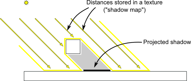
Rendering the shadow map
In this tutorial, we’ll only consider directional lights - lights that are so far away that all the light rays can be considered parallel. As such, rendering the shadow map is done with an orthographic projection matrix. An orthographic matrix is just like a usual perspective projection matrix, except that no perspective is taken into account - an object will look the same whether it’s far or near the camera.
Setting up the rendertarget and the MVP matrix
Since Tutorial 14, you know how to render the scene into a texture in order to access it later from a shader.
Here we use a 1024x1024 16-bit depth texture to contain the shadow map. 16 bits are usually enough for a shadow map. Feel free to experiment with these values. Note that we use a depth texture, not a depth renderbuffer, since we’ll need to sample it later.
// The framebuffer, which regroups 0, 1, or more textures, and 0 or 1 depth buffer.
 GLuint FramebufferName = 0;
 glGenFramebuffers(1, &FramebufferName);
 glBindFramebuffer(GL_FRAMEBUFFER, FramebufferName);

 // Depth texture. Slower than a depth buffer, but you can sample it later in your shader
 GLuint depthTexture;
 glGenTextures(1, &depthTexture);
 glBindTexture(GL_TEXTURE_2D, depthTexture);
 glTexImage2D(GL_TEXTURE_2D, 0,GL_DEPTH_COMPONENT16, 1024, 1024, 0,GL_DEPTH_COMPONENT, GL_FLOAT, 0);
 glTexParameteri(GL_TEXTURE_2D, GL_TEXTURE_MAG_FILTER, GL_NEAREST);
 glTexParameteri(GL_TEXTURE_2D, GL_TEXTURE_MIN_FILTER, GL_NEAREST);
 glTexParameteri(GL_TEXTURE_2D, GL_TEXTURE_WRAP_S, GL_CLAMP_TO_EDGE);
 glTexParameteri(GL_TEXTURE_2D, GL_TEXTURE_WRAP_T, GL_CLAMP_TO_EDGE);

 glFramebufferTexture(GL_FRAMEBUFFER, GL_DEPTH_ATTACHMENT, depthTexture, 0);

 glDrawBuffer(GL_NONE); // No color buffer is drawn to.

 // Always check that our framebuffer is ok
 if(glCheckFramebufferStatus(GL_FRAMEBUFFER) != GL_FRAMEBUFFER_COMPLETE)
 return false;
The MVP matrix used to render the scene from the light’s point of view is computed as follows :
- The Projection matrix is an orthographic matrix which will encompass everything in the axis-aligned box (-10,10),(-10,10),(-10,20) on the X,Y and Z axes respectively. These values are made so that our entire *visible *scene is always visible ; more on this in the Going Further section.
- The View matrix rotates the world so that in camera space, the light direction is -Z (would you like to re-read Tutorial 3 ?)
- The Model matrix is whatever you want.
glm::vec3 lightInvDir = glm::vec3(0.5f,2,2);

 // Compute the MVP matrix from the light's point of view
 glm::mat4 depthProjectionMatrix = glm::ortho<float>(-10,10,-10,10,-10,20);
 glm::mat4 depthViewMatrix = glm::lookAt(lightInvDir, glm::vec3(0,0,0), glm::vec3(0,1,0));
 glm::mat4 depthModelMatrix = glm::mat4(1.0);
 glm::mat4 depthMVP = depthProjectionMatrix * depthViewMatrix * depthModelMatrix;

 // Send our transformation to the currently bound shader,
 // in the "MVP" uniform
 glUniformMatrix4fv(depthMatrixID, 1, GL_FALSE, &depthMVP[0][0])
The shaders
The shaders used during this pass are very simple. The vertex shader is a pass-through shader which simply compute the vertex’ position in homogeneous coordinates :
#version 330 core

// Input vertex data, different for all executions of this shader.
layout(location = 0) in vec3 vertexPosition_modelspace;

// Values that stay constant for the whole mesh.
uniform mat4 depthMVP;

void main(){
 gl_Position =  depthMVP * vec4(vertexPosition_modelspace,1);
}
The fragment shader is just as simple : it simply writes the depth of the fragment at location 0 (i.e. in our depth texture).
#version 330 core

// Ouput data
layout(location = 0) out float fragmentdepth;

void main(){
    // Not really needed, OpenGL does it anyway
    fragmentdepth = gl_FragCoord.z;
}
Rendering a shadow map is usually more than twice as fast as the normal render, because only low precision depth is written, instead of both the depth and the color; Memory bandwidth is often the biggest performance issue on GPUs.
Result
The resulting texture looks like this :

A dark colour means a small z ; hence, the upper-right corner of the wall is near the camera. At the opposite, white means z=1 (in homogeneous coordinates), so this is very far.
Using the shadow map
Basic shader
Now we go back to our usual shader. For each fragment that we compute, we must test whether it is “behind” the shadow map or not.
To do this, we need to compute the current fragment’s position in the same space that the one we used when creating the shadowmap. So we need to transform it once with the usual MVP matrix, and another time with the depthMVP matrix.
There is a little trick, though. Multiplying the vertex’ position by depthMVP will give homogeneous coordinates, which are in [-1,1] ; but texture sampling must be done in [0,1].
For instance, a fragment in the middle of the screen will be in (0,0) in homogeneous coordinates ; but since it will have to sample the middle of the texture, the UVs will have to be (0.5, 0.5).
This can be fixed by tweaking the fetch coordinates directly in the fragment shader but it’s more efficient to multiply the homogeneous coordinates by the following matrix, which simply divides coordinates by 2 ( the diagonal : [-1,1] -> [-0.5, 0.5] ) and translates them ( the lower row : [-0.5, 0.5] -> [0,1] ).
glm::mat4 biasMatrix(
0.5, 0.0, 0.0, 0.0,
0.0, 0.5, 0.0, 0.0,
0.0, 0.0, 0.5, 0.0,
0.5, 0.5, 0.5, 1.0
);
glm::mat4 depthBiasMVP = biasMatrix*depthMVP;
We can now write our vertex shader. It’s the same as before, but we output 2 positions instead of 1 :
- gl_Position is the position of the vertex as seen from the current camera
- ShadowCoord is the position of the vertex as seen from the last camera (the light)
// Output position of the vertex, in clip space : MVP * position
gl_Position =  MVP * vec4(vertexPosition_modelspace,1);

// Same, but with the light's view matrix
ShadowCoord = DepthBiasMVP * vec4(vertexPosition_modelspace,1);
The fragment shader is then very simple :
- texture( shadowMap, ShadowCoord.xy ).z is the distance between the light and the nearest occluder
- ShadowCoord.z is the distance between the light and the current fragment
… so if the current fragment is further than the nearest occluder, this means we are in the shadow (of said nearest occluder) :
float visibility = 1.0;
if ( texture( shadowMap, ShadowCoord.xy ).z  <  ShadowCoord.z){
    visibility = 0.5;
}
We just have to use this knowledge to modify our shading. Of course, the ambient colour isn’t modified, since its purpose in life is to fake some incoming light even when we’re in the shadow (or everything would be pure black)
color =
 // Ambient : simulates indirect lighting
 MaterialAmbientColor +
 // Diffuse : "color" of the object
 visibility * MaterialDiffuseColor * LightColor * LightPower * cosTheta+
 // Specular : reflective highlight, like a mirror
 visibility * MaterialSpecularColor * LightColor * LightPower * pow(cosAlpha,5);
Result - Shadow acne
Here’s the result of the current code. Obviously, the global idea it there, but the quality is unacceptable.
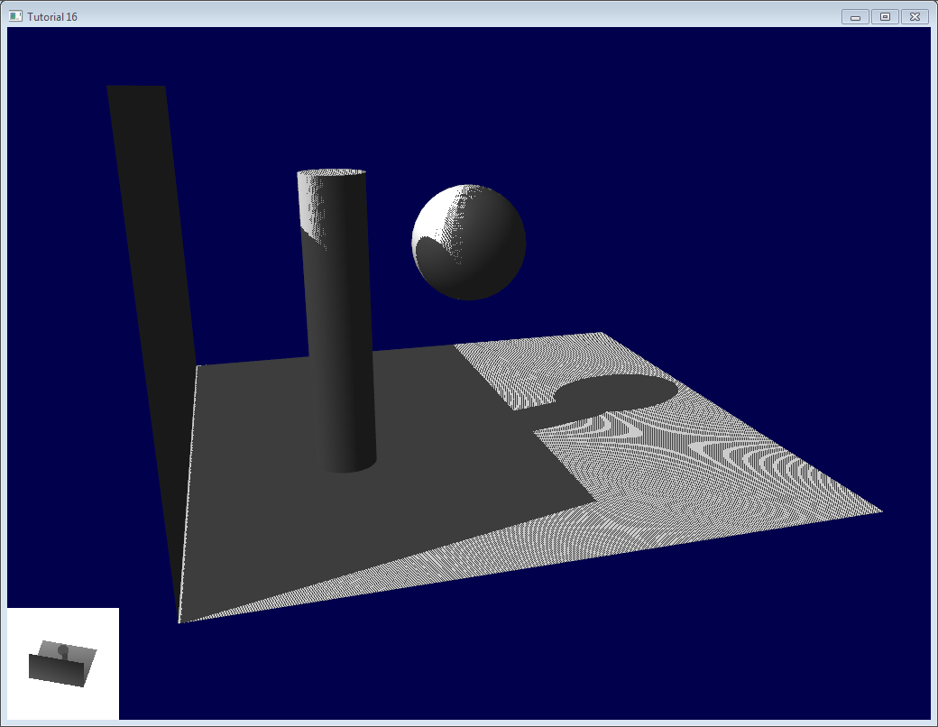
Let’s look at each problem in this image. The code has 2 projects : shadowmaps and shadowmaps_simple; start with whichever you like best. The simple version is just as ugly as the image above, but is simpler to understand.
Problems
Shadow acne
The most obvious problem is called shadow acne :
This phenomenon is easily explained with a simple image :
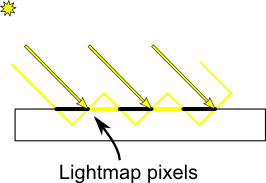
The usual “fix” for this is to add an error margin : we only shade if the current fragment’s depth (again, in light space) is really far away from the lightmap value. We do this by adding a bias :
float bias = 0.005;
float visibility = 1.0;
if ( texture( shadowMap, ShadowCoord.xy ).z  <  ShadowCoord.z-bias){
    visibility = 0.5;
}
The result is already much nicer :
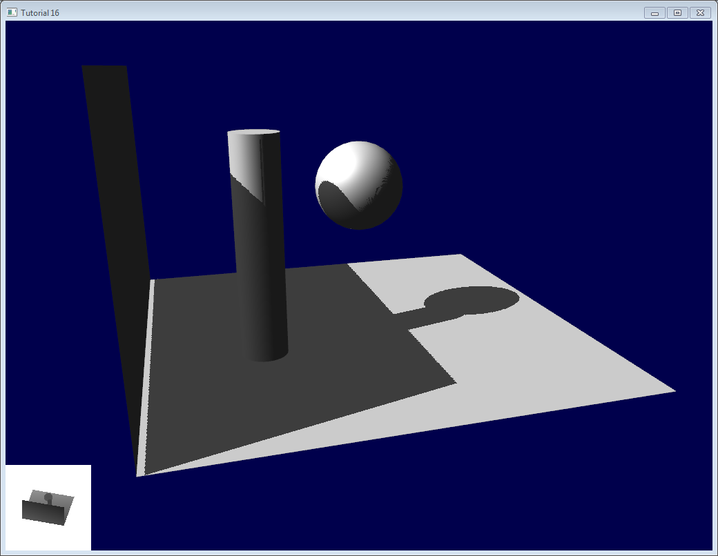
However, you can notice that because of our bias, the artefact between the ground and the wall has gone worse. What’s more, a bias of 0.005 seems too much on the ground, but not enough on curved surface : some artefacts remain on the cylinder and on the sphere.
A common approach is to modify the bias according to the slope :
float bias = 0.005*tan(acos(cosTheta)); // cosTheta is dot( n,l ), clamped between 0 and 1
bias = clamp(bias, 0,0.01);
Shadow acne is now gone, even on curved surfaces.

Another trick, which may or may not work depending on your geometry, is to render only the back faces in the shadow map. This forces us to have a special geometry ( see next section - Peter Panning ) with thick walls, but at least, the acne will be on surfaces which are in the shadow :
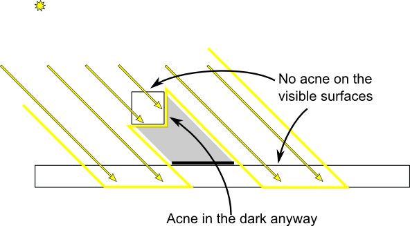
When rendering the shadow map, cull front-facing triangles :
        // We don't use bias in the shader, but instead we draw back faces,
        // which are already separated from the front faces by a small distance
        // (if your geometry is made this way)
        glCullFace(GL_FRONT); // Cull front-facing triangles -> draw only back-facing triangles
And when rendering the scene, render normally (backface culling)
glCullFace(GL_BACK); // Cull back-facing triangles -> draw only front-facing triangles
This method is used in the code, in addition to the bias.
Peter Panning
We have no shadow acne anymore, but we still have this wrong shading of the ground, making the wall to look as if it’s flying (hence the term “Peter Panning”). In fact, adding the bias made it worse.
This one is very easy to fix : simply avoid thin geometry. This has two advantages :
- First, it solves Peter Panning : it the geometry is more deep than your bias, you’re all set.
- Second, you can turn on backface culling when rendering the lightmap, because now, there is a polygon of the wall which is facing the light, which will occlude the other side, which wouldn’t be rendered with backface culling.
The drawback is that you have more triangles to render ( two times per frame ! )

Aliasing
Even with these two tricks, you’ll notice that there is still aliasing on the border of the shadow. In other words, one pixel is white, and the next is black, without a smooth transition inbetween.

PCF
The easiest way to improve this is to change the shadowmap’s sampler type to sampler2DShadow. The consequence is that when you sample the shadowmap once, the hardware will in fact also sample the neighboring texels, do the comparison for all of them, and return a float in [0,1] with a bilinear filtering of the comparison results.
For instance, 0.5 means that 2 samples are in the shadow, and 2 samples are in the light.
Note that it’s not the same than a single sampling of a filtered depth map ! A comparison always returns true or false; PCF gives a interpolation of 4 “true or false”.

As you can see, shadow borders are smooth, but shadowmap’s texels are still visible.
Poisson Sampling
An easy way to deal with this is to sample the shadowmap N times instead of once. Used in combination with PCF, this can give very good results, even with a small N. Here’s the code for 4 samples :
for (int i=0;i<4;i++){
  if ( texture( shadowMap, ShadowCoord.xy + poissonDisk[i]/700.0 ).z  <  ShadowCoord.z-bias ){
    visibility-=0.2;
  }
}
poissonDisk is a constant array defines for instance as follows :
vec2 poissonDisk[4] = vec2[](
  vec2( -0.94201624, -0.39906216 ),
  vec2( 0.94558609, -0.76890725 ),
  vec2( -0.094184101, -0.92938870 ),
  vec2( 0.34495938, 0.29387760 )
);
This way, depending on how many shadowmap samples will pass, the generated fragment will be more or less dark :
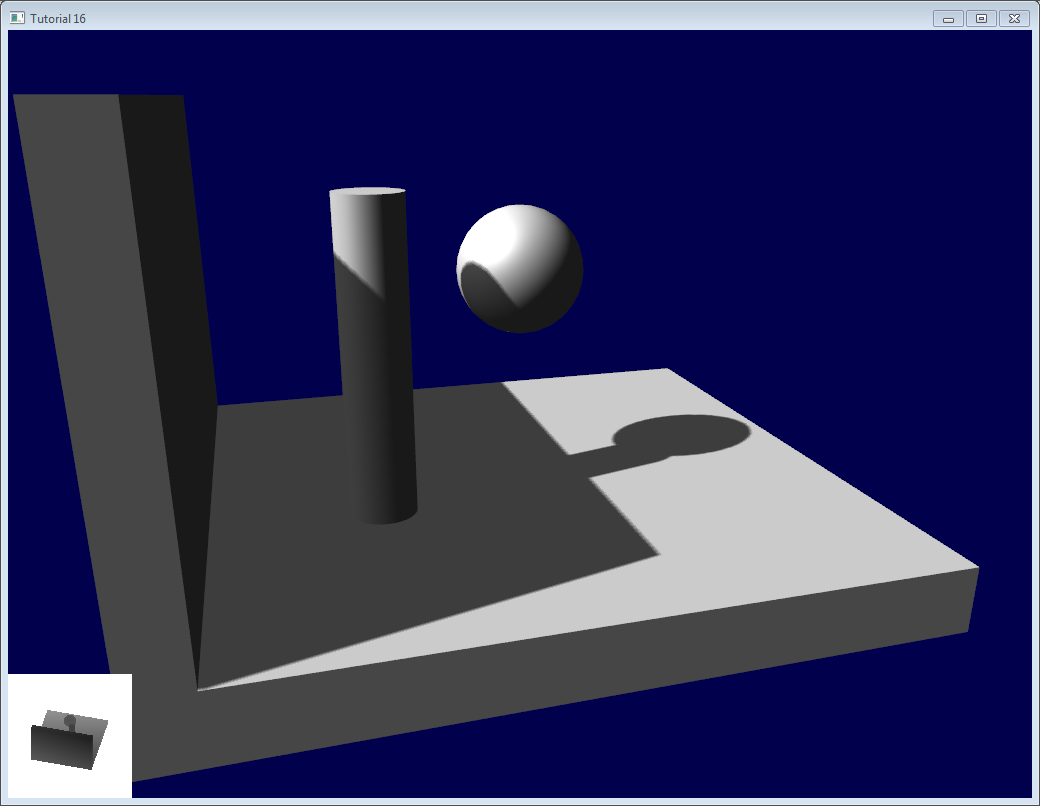
The 700.0 constant defines how much the samples are “spread”. Spread them too little, and you’ll get aliasing again; too much, and you’ll get this :* banding (this screenshot doesn’t use PCF for a more dramatic effect, but uses 16 samples instead) *

Stratified Poisson Sampling
We can remove this banding by choosing different samples for each pixel. There are two main methods : Stratified Poisson or Rotated Poisson. Stratified chooses different samples; Rotated always use the same, but with a random rotation so that they look different. In this tutorial I will only explain the stratified version.
The only difference with the previous version is that we index poissonDisk with a random index :
    for (int i=0;i<4;i++){
        int index = // A random number between 0 and 15, different for each pixel (and each i !)
        visibility -= 0.2*(1.0-texture( shadowMap, vec3(ShadowCoord.xy + poissonDisk[index]/700.0,  (ShadowCoord.z-bias)/ShadowCoord.w) ));
    }
We can generate a random number with a code like this, which returns a random number in [0,1[ :
    float dot_product = dot(seed4, vec4(12.9898,78.233,45.164,94.673));
    return fract(sin(dot_product) * 43758.5453);
In our case, seed4 will be the combination of i (so that we sample at 4 different locations) and … something else. We can use gl_FragCoord ( the pixel’s location on the screen ), or Position_worldspace :
        //  - A random sample, based on the pixel's screen location.
        //    No banding, but the shadow moves with the camera, which looks weird.
        int index = int(16.0*random(gl_FragCoord.xyy, i))%16;
        //  - A random sample, based on the pixel's position in world space.
        //    The position is rounded to the millimeter to avoid too much aliasing
        //int index = int(16.0*random(floor(Position_worldspace.xyz*1000.0), i))%16;
This will make patterns such as in the picture above disappear, at the expense of visual noise. Still, a well-done noise is often less objectionable than these patterns.
See tutorial16/ShadowMapping.fragmentshader for three example implementions.
Going further
Even with all these tricks, there are many, many ways in which our shadows could be improved. Here are the most common :
Early bailing
Instead of taking 16 samples for each fragment (again, it’s a lot), take 4 distant samples. If all of them are in the light or in the shadow, you can probably consider that all 16 samples would have given the same result : bail early. If some are different, you’re probably on a shadow boundary, so the 16 samples are needed.
Spot lights
Dealing with spot lights requires very few changes. The most obvious one is to change the orthographic projection matrix into a perspective projection matrix :
glm::vec3 lightPos(5, 20, 20);
glm::mat4 depthProjectionMatrix = glm::perspective<float>(glm::radians(45.0f), 1.0f, 2.0f, 50.0f);
glm::mat4 depthViewMatrix = glm::lookAt(lightPos, lightPos-lightInvDir, glm::vec3(0,1,0));
same thing, but with a perspective frustum instead of an orthographic frustum. Use texture2Dproj to account for perspective-divide (see footnotes in tutorial 4 - Matrices)
The second step is to take into account the perspective in the shader. (see footnotes in tutorial 4 - Matrices. In a nutshell, a perspective projection matrix actually doesn’t do any perspective at all. This is done by the hardware, by dividing the projected coordinates by w. Here, we emulate the transformation in the shader, so we have to do the perspective-divide ourselves. By the way, an orthographic matrix always generates homogeneous vectors with w=1, which is why they don’t produce any perspective)
Here are two way to do this in GLSL. The second uses the built-in textureProj function, but both methods produce exactly the same result.
if ( texture( shadowMap, (ShadowCoord.xy/ShadowCoord.w) ).z  <  (ShadowCoord.z-bias)/ShadowCoord.w )
if ( textureProj( shadowMap, ShadowCoord.xyw ).z  <  (ShadowCoord.z-bias)/ShadowCoord.w )
Point lights
Same thing, but with depth cubemaps. A cubemap is a set of 6 textures, one on each side of a cube; what’s more, it is not accessed with standard UV coordinates, but with a 3D vector representing a direction.
The depth is stored for all directions in space, which make possible for shadows to be cast all around the point light.
Combination of several lights
The algorithm handles several lights, but keep in mind that each light requires an additional rendering of the scene in order to produce the shadowmap. This will require an enormous amount of memory when applying the shadows, and you might become bandwidth-limited very quickly.
Automatic light frustum
In this tutorial, the light frustum hand-crafted to contain the whole scene. While this works in this restricted example, it should be avoided. If your map is 1Km x 1Km, each texel of your 1024x1024 shadowmap will take 1 square meter; this is lame. The projection matrix of the light should be as tight as possible.
For spot lights, this can be easily changed by tweaking its range.
Directional lights, like the sun, are more tricky : they really do illuminate the whole scene. Here’s a way to compute a the light frustum :
-
Potential Shadow Receivers, or PSRs for short, are objects which belong at the same time to the light frustum, to the view frustum, and to the scene bounding box. As their name suggest, these objects are susceptible to be shadowed : they are visible by the camera and by the light.
-
Potential Shadow Casters, or PCFs, are all the Potential Shadow Receivers, plus all objects which lie between them and the light (an object may not be visible but still cast a visible shadow).
So, to compute the light projection matrix, take all visible objects, remove those which are too far away, and compute their bounding box; Add the objects which lie between this bounding box and the light, and compute the new bounding box (but this time, aligned along the light direction).
Precise computation of these sets involve computing convex hulls intersections, but this method is much easier to implement.
This method will result in popping when objects disappear from the frustum, because the shadowmap resolution will suddenly increase. Cascaded Shadow Maps don’t have this problem, but are harder to implement, and you can still compensate by smoothing the values over time.
Exponential shadow maps
Exponential shadow maps try to limit aliasing by assuming that a fragment which is in the shadow, but near the light surface, is in fact “somewhere in the middle”. This is related to the bias, except that the test isn’t binary anymore : the fragment gets darker and darker when its distance to the lit surface increases.
This is cheating, obviously, and artefacts can appear when two objects overlap.
Light-space perspective Shadow Maps
LiSPSM tweaks the light projection matrix in order to get more precision near the camera. This is especially important in case of “duelling frustra” : you look in a direction, but a spot light “looks” in the opposite direction. You have a lot of shadowmap precision near the light, i.e. far from you, and a low resolution near the camera, where you need it the most.
However LiSPM is tricky to implement. See the references for details on the implementation.
Cascaded shadow maps
CSM deals with the exact same problem than LiSPSM, but in a different way. It simply uses several (2-4) standard shadow maps for different parts of the view frustum. The first one deals with the first meters, so you’ll get great resolution for a quite little zone. The next shadowmap deals with more distant objects. The last shadowmap deals with a big part of the scene, but due tu the perspective, it won’t be more visually important than the nearest zone.
Cascarded shadow maps have, at time of writing (2012), the best complexity/quality ratio. This is the solution of choice in many cases.
Conclusion
As you can see, shadowmaps are a complex subject. Every year, new variations and improvement are published, and to day, no solution is perfect.
Fortunately, most of the presented methods can be mixed together : It’s perfectly possible to have Cascaded Shadow Maps in Light-space Perspective, smoothed with PCF… Try experimenting with all these techniques.
As a conclusion, I’d suggest you to stick to pre-computed lightmaps whenever possible, and to use shadowmaps only for dynamic objects. And make sure that the visual quality of both are equivalent : it’s not good to have a perfect static environment and ugly dynamic shadows, either.
Tutorial 17 : Rotations
- Foreword: rotation VS orientation
- Euler Angles
- Quaternions
- So, which one should I choose ?
- Other resources
- Cheat-sheet
- How do I know if two quaternions are similar ?
- How do I apply a rotation to a point ?
- How do I interpolate between 2 quaternions ?
- How do I cumulate 2 rotations ?
- How do I find the rotation between 2 vectors ?
- I need an equivalent of gluLookAt. How do I orient an object towards a point ?
- How do I use LookAt, but limit the rotation at a certain speed ?
- How do I…
This tutorial goes a bit outside the scope of OpenGL, but nevertheless tackles a very common problem: how to represent rotations ?
In Tutorial 3 - Matrices, we learnt that matrices are able to rotate a point around a specific axis. While matrices are a neat way to transform vertices, handling matrices is difficult: for instance, getting the rotation axis from the final matrix is quite tricky.
We will present the two most common ways to represent rotation: Euler angles and Quaternions. Most importantly, we will explain why you should probably use Quaternions.
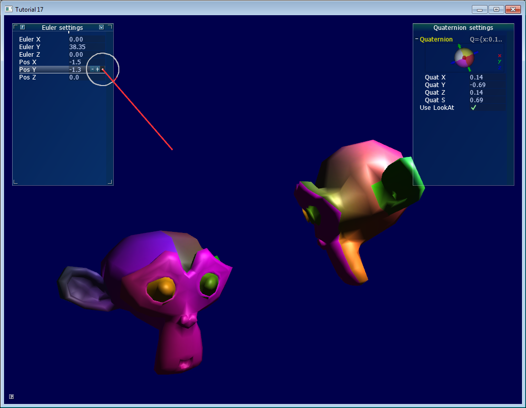
Foreword: rotation VS orientation
While reading articles on rotations, you might get confused because of the vocabulary. In this tutorial:
- An orientation is a state: “the object’s orientation is…”
- A rotation is an operation: “Apply this rotation to the object”
That is, when you apply a rotation, you change the orientation. Both can be represented with the same tools, which leads to the confusion. Now, let’s get started…
Euler Angles
Euler angles are the easiest way to think of an orientation. You basically store three rotations around the X, Y and Z axes. It’s a very simple concept to grasp. You can use a vec3 to store it:
vec3 EulerAngles( RotationAroundXInRadians, RotationAroundYInRadians, RotationAroundZInRadians);
These 3 rotations are then applied successively, usually in this order: first Y, then Z, then X (but not necessarily). Using a different order yields different results.
One simple use of Euler angles is setting a character’s orientation. Usually game characters do not rotate on X and Z, only on the vertical axis. Therefore, it’s easier to write, understand and maintain “float direction;” than 3 different orientations.
Another good use of Euler angles is an FPS camera: you have one angle for the heading (Y), and one for up/down (X). See common/controls.cpp for an example.
However, when things get more complex, Euler angle will be hard to work with. For instance :
- Interpolating smoothly between 2 orientations is hard. Naively interpolating the X,Y and Z angles will be ugly.
- Applying several rotations is complicated and unprecise: you have to compute the final rotation matrix, and guess the Euler angles from this matrix
- A well-known problem, the “Gimbal Lock”, will sometimes block your rotations, and other singularities which will flip your model upside-down.
- Different angles make the same rotation ( -180° and 180°, for instance )
- It’s a mess - as said above, usually the right order is YZX, but if you also use a library with a different order, you’ll be in trouble.
- Some operations are complicated: for instance, rotation of N degrees around a specific axis.
Quaternions are a tool to represent rotations, which solves these problems.
Quaternions
A quaternion is a set of 4 numbers, [x y z w], which represents rotations the following way:
// RotationAngle is in radians
x = RotationAxis.x * sin(RotationAngle / 2)
y = RotationAxis.y * sin(RotationAngle / 2)
z = RotationAxis.z * sin(RotationAngle / 2)
w = cos(RotationAngle / 2)
RotationAxis is, as its name implies, the axis around which you want to make your rotation.
RotationAngle is the angle of rotation around this axis.
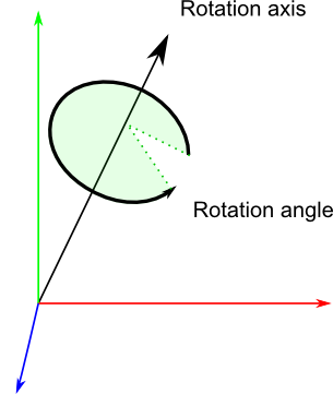
So essentially quaternions store a rotation axis and a rotation angle, in a way that makes combining rotations easy.
Reading quaternions
This format is definitely less intuitive than Euler angles, but it’s still readable: the xyz components match roughly the rotation axis, and the acos of w is the rotation angle (divided by 2). For instance, imagine that you see the following values in the debugger: [ 0.7 0 0 0.7 ]. x=0.7, it’s bigger than y and z, so you know it’s mostly a rotation around the X axis; and 2*acos(0.7) = 1.59 radians, so it’s a rotation of 90°.
Similarly, [0 0 0 1] (w=1) means that angle = 2*acos(1) = 0, so this is a unit quaternion, which makes no rotation at all.
Basic operations
Knowing the math behind the quaternions is rarely useful: the representation is so unintuitive that you usually only rely on utility functions which do the math for you. If you’re interested, see the math books in the Useful Tools & Links page.
How do I create a quaternion in C++ ?
// Don't forget to #include <glm/gtc/quaternion.hpp> and <glm/gtx/quaternion.hpp>

// Creates an identity quaternion (no rotation)
quat MyQuaternion;

// Direct specification of the 4 components
// You almost never use this directly
MyQuaternion = quat(w,x,y,z);

// Conversion from Euler angles (in radians) to Quaternion
vec3 EulerAngles(90, 45, 0);
MyQuaternion = quat(EulerAngles);

// Conversion from axis-angle
// In GLM the angle must be in degrees here, so convert it.
MyQuaternion = gtx::quaternion::angleAxis(degrees(RotationAngle), RotationAxis);
How do I create a quaternion in GLSL ?
You don’t. Convert your quaternion to a rotation matrix, and use it in the Model Matrix. Your vertices will be rotated as usual, with the MVP matrix.
In some cases, you might actually want to use quaternions in GLSL, for instance if you do skeletal animation on the GPU. There is no quaternion type in GLSL, but you can pack one in a vec4, and do the math yourself in the shader.
How do I convert a quaternion to a matrix ?
mat4 RotationMatrix = quaternion::toMat4(quaternion);
You can now use it to build your Model matrix as usual:
mat4 RotationMatrix = quaternion::toMat4(quaternion);
...
mat4 ModelMatrix = TranslationMatrix * RotationMatrix * ScaleMatrix;
// You can now use ModelMatrix to build the MVP matrix
So, which one should I choose ?
Choosing between Euler angles and quaternions is tricky. Euler angles are intuitive for artists, so if you write some 3D editor, use them. But quaternions are handy for programmers, and faster too, so you should use them in a 3D engine core.
The general consensus is exactly that: use quaternions internally, and expose Euler angles whenever you have some kind of user interface.
You will be able to handle all you will need (or at least, it will be easier), and you can still use Euler angles for entities that require it ( as said above: the camera, humanoids, and that’s pretty much it) with a simple conversion.
Other resources
- The books on Useful Tools & Links !
- As old as it can be, Game Programming Gems 1 has several awesome articles on quaternions. You can probably find them online too.
- A GDC presentation on rotations
- Ogre3D’s FAQ on quaternions. Most of the 2nd part is ogre-specific, though.
- Ogre3D’s Vector3D.h and Quaternion.cpp
Cheat-sheet
How do I know if two quaternions are similar ?
When using vector, the dot product gives the cosine of the angle between these vectors. If this value is 1, then the vectors are in the same direction.
With quaternions, it’s exactly the same:
float matching = quaternion::dot(q1, q2);
if ( abs(matching-1.0) < 0.001 ){
    // q1 and q2 are similar
}
You can also get the angle between q1 and q2 by taking the acos() of this dot product.
How do I apply a rotation to a point ?
You can do the following:
rotated_point = orientation_quaternion * point;
… but if you want to compute your Model Matrix, you should probably convert it to a matrix instead.
Note that the center of rotation is always the origin. If you want to rotate around another point:
rotated_point = origin + (orientation_quaternion * (point-origin));
How do I interpolate between 2 quaternions ?
This is called a SLERP: Spherical Linear intERPolation. With GLM, you can do this with mix:
glm::quat interpolatedquat = quaternion::mix(quat1, quat2, 0.5f); // or whatever factor
How do I cumulate 2 rotations ?
Simple ! Just multiply the two quaternions together. The order is the same as for matrices, i.e. reverse:
quat combined_rotation = second_rotation * first_rotation;
How do I find the rotation between 2 vectors ?
(in other words: the quaternion needed to rotate v1 so that it matches v2)
The basic idea is straightforward:
- The angle between the vectors is simple to find: the dot product gives its cosine.
- The needed axis is also simple to find: it’s the cross product of the two vectors.
The following algorithm does exactly this, but also handles a number of special cases:
quat RotationBetweenVectors(vec3 start, vec3 dest){
	start = normalize(start);
	dest = normalize(dest);

	float cosTheta = dot(start, dest);
	vec3 rotationAxis;

	if (cosTheta < -1 + 0.001f){
		// special case when vectors in opposite directions:
		// there is no "ideal" rotation axis
		// So guess one; any will do as long as it's perpendicular to start
		rotationAxis = cross(vec3(0.0f, 0.0f, 1.0f), start);
		if (gtx::norm::length2(rotationAxis) < 0.01 ) // bad luck, they were parallel, try again!
			rotationAxis = cross(vec3(1.0f, 0.0f, 0.0f), start);

		rotationAxis = normalize(rotationAxis);
		return gtx::quaternion::angleAxis(glm::radians(180.0f), rotationAxis);
	}

	rotationAxis = cross(start, dest);

	float s = sqrt( (1+cosTheta)*2 );
	float invs = 1 / s;

	return quat(
		s * 0.5f,
		rotationAxis.x * invs,
		rotationAxis.y * invs,
		rotationAxis.z * invs
	);

}
(You can find this function in common/quaternion_utils.cpp)
I need an equivalent of gluLookAt. How do I orient an object towards a point ?
Use RotationBetweenVectors !
// Find the rotation between the front of the object (that we assume towards +Z,
// but this depends on your model) and the desired direction
quat rot1 = RotationBetweenVectors(vec3(0.0f, 0.0f, 1.0f), direction);
Now, you might also want to force your object to be upright:
// Recompute desiredUp so that it's perpendicular to the direction
// You can skip that part if you really want to force desiredUp
vec3 right = cross(direction, desiredUp);
desiredUp = cross(right, direction);

// Because of the 1rst rotation, the up is probably completely screwed up.
// Find the rotation between the "up" of the rotated object, and the desired up
vec3 newUp = rot1 * vec3(0.0f, 1.0f, 0.0f);
quat rot2 = RotationBetweenVectors(newUp, desiredUp);
Now, combine them:
quat targetOrientation = rot2 * rot1; // remember, in reverse order.
Beware, “direction” is, well, a direction, not the target position ! But you can compute the position simply: targetPos - currentPos.
Once you have this target orientation, you will probably want to interpolate between startOrientation and targetOrientation.
(You can find this function in common/quaternion_utils.cpp)
How do I use LookAt, but limit the rotation at a certain speed ?
The basic idea is to do a SLERP ( = use glm::mix ), but play with the interpolation value so that the angle is not bigger than the desired value:
float mixFactor = maxAllowedAngle / angleBetweenQuaternions;
quat result = glm::gtc::quaternion::mix(q1, q2, mixFactor);
Here is a more complete implementation, which deals with many special cases. Note that it doesn’t use mix() directly as an optimization.
quat RotateTowards(quat q1, quat q2, float maxAngle){
if( maxAngle < 0.001f ){
// No rotation allowed. Prevent dividing by 0 later.
return q1;
}
float cosTheta = dot(q1, q2);
// q1 and q2 are already equal.
// Force q2 just to be sure
if(cosTheta > 0.9999f){
return q2;
}
// Avoid taking the long path around the sphere
if (cosTheta < 0){
q1 = q1*-1.0f;
cosTheta *= -1.0f;
}
float angle = acos(cosTheta);
// If there is only a 2° difference, and we are allowed 5°,
// then we arrived.
if (angle < maxAngle){
return q2;
}
float fT = maxAngle / angle;
angle = maxAngle;
quat res = (sin((1.0f - fT) * angle) * q1 + sin(fT * angle) * q2) / sin(angle);
res = normalize(res);
return res;
}
You can use it like that:
CurrentOrientation = RotateTowards(CurrentOrientation, TargetOrientation, 3.14f * deltaTime );
(You can find this function in common/quaternion_utils.cpp)
How do I…
If you can’t figure it out, drop us an email, and we’ll add it to the list !
Billboards
- Solution #1 : The 2D way
- Solution #2 : The 3D way
- Solution #3 : The fixed-size 3D way
- Solution #4 : Vertical rotation only
Billboards are 2D elements incrusted in a 3D world. Not a 2D menu on top of everything else; not a 3D plane around which you can turn; but something in-between, like health bars in many games.
What’s different with billboards is that they are positionned at a specific location, but their orientation is automatically computed so that it always faces the camera.
Solution #1 : The 2D way
This one is supra-easy.
Just compute where your point is on screen, and display a 2D text (see Tutorial 11) at this position.
// Everything here is explained in Tutorial 3 ! There's nothing new.
glm::vec4 BillboardPos_worldspace(x,y,z, 1.0f);
glm::vec4 BillboardPos_screenspace = ProjectionMatrix * ViewMatrix * BillboardPos_worldspace;
BillboardPos_screenspace /= BillboardPos_screenspace.w;

if (BillboardPos_screenspace.z < 0.0f){
    // Object is behind the camera, don't display it.
}
Ta-dah !
On the plus side, this method is really easy, and the billboard will have the same size regardless of its distance to the camera. But 2D text is always displayed on top of everything else, and this can/will mess up the rendering and show above other objects.
Solution #2 : The 3D way
This one is usually better and not much more complicated.
The goal is to keep the mesh aligned with the camera, even when the camera moves :
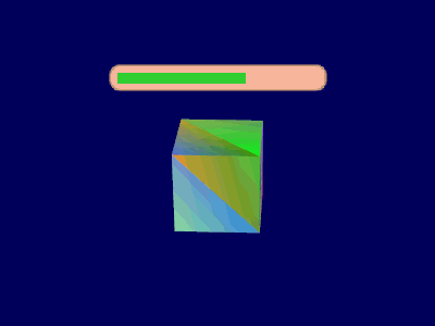
You can view this problem as generating an appropriate Model matrix, even though it’s is much simpler than that.
The idea is that each corner of the billboard is at the center position, displaced by the camera’s up and right vectors :
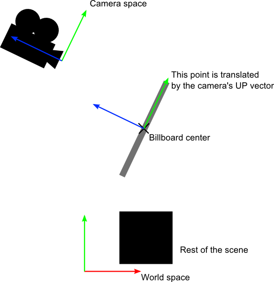
Of course, we only know the billboard’s center position in world space, so we also need the camera’s up/right vectors in world space.
In camera space, the camera’s up vector is (0,1,0). To get it in world space, just multiply this by the matrix that goes from Camera Space to World Space, which is, of course, the inverse of the View matrix.
An easier way to express the same math is :
CameraRight_worldspace = {ViewMatrix[0][0], ViewMatrix[1][0], ViewMatrix[2][0]}
CameraUp_worldspace = {ViewMatrix[0][1], ViewMatrix[1][1], ViewMatrix[2][1]}
Once we have this, it’s very easy to compute the final vertex’ position :
vec3 vertexPosition_worldspace =
    particleCenter_wordspace
    + CameraRight_worldspace * squareVertices.x * BillboardSize.x
    + CameraUp_worldspace * squareVertices.y * BillboardSize.y;
- particleCenter_worldspace is, as its name suggests, the billboard’s center position. It is specified with an uniform vec3.
- squareVertices is the original mesh. squareVertices.x is -0.5 for the left vertices, which are thus moved towars the left of the camera (because of the *CameraRight_worldspace)
- BillboardSize is the size, in world units, of the billboard, sent as another uniform.

For the record, here’s how squareVertices is made :
// The VBO containing the 4 vertices of the particles.
 static const GLfloat g_vertex_buffer_data[] = {
 -0.5f, -0.5f, 0.0f,
 0.5f, -0.5f, 0.0f,
 -0.5f, 0.5f, 0.0f,
 0.5f, 0.5f, 0.0f,
 };
Solution #3 : The fixed-size 3D way
As you can see above, the size of the billboard changes with respect to the camera’s distance. This is the expected result in some cases, but in others, such as health bars, you probably want a fixed-size instead.
Since the displacement between the center and a corner must be fixed in screen-space, that’s exactly what we’re going to do : compute the center’s position in screen space, and offset it.
vertexPosition_worldspace = particleCenter_wordspace;
// Get the screen-space position of the particle's center
gl_Position = VP * vec4(vertexPosition_worldspace, 1.0f);
// Here we have to do the perspective division ourselves.
gl_Position /= gl_Position.w;

// Move the vertex in directly screen space. No need for CameraUp/Right_worlspace here.
gl_Position.xy += squareVertices.xy * vec2(0.2, 0.05);
Remember that at this stage of the rendering pipeline, you’re in Normalized Device Coordinates, so between -1 and 1 on both axes : it’s not in pixels.
If you want a size in pixels, easy : just use (ScreenSizeInPixels / BillboardSizeInPixels) instead of BillboardSizeInScreenPercentage.
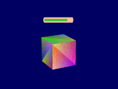
Solution #4 : Vertical rotation only
Some systems model faraway trees and lamps as billboards. But you really, really don’t want your tree to be bent : it MUST be vertical. So you need an hybrid system that rotates only around one axis.
Well, this one is left as an exercise to the reader !
Particles / Instancing
Particles are very similar to 3D billboards. There are two major differences, though :
- there is usually a LOT of them
- they move
- the appear and die.
- they are semi-transparent
Both of these difference come with problems. This tutorial will present ONE way to solve them; there are many other possibilities.
Particles, lots of them !
The first idea to draw many particles would be to use the previous tutorial’s code, and call glDrawArrays once for each particle. This is a very bad idea, because this means that all your shiny GTX’ 512+ multiprocessors will all be dedicated to draw ONE quad (obviously, only one will be used, so that’s 99% efficiency loss). Then you will draw the second billboard, and it will be the same.
Clearly, we need a way to draw all particles at the same time.
There are many ways to do this; here are three of them :
- Generate a single VBO with all the particles in them. Easy, effective, works on all platforms.
- Use geometry shaders. Not in the scope of this tutorial, mostly because 50% of the computers don’t support this.
- Use instancing. Not available on ALL computers, but a vast majority of them.
In this tutorial, we’ll use the 3rd option, because it is a nice balance between performance and availability, and on top of that, it’s easy to add support for the first method once this one works.
Instancing
“Instancing” means that we have a base mesh (in our case, a simple quad of 2 triangles), but many instances of this quad.
Technically, it’s done via several buffers :
- Some of them describe the base mesh
- Some of them describe the particularities of each instance of the base mesh.
You have many, many options on what to put in each buffer. In our simple case, we have :
- One buffer for the vertices of the mesh. No index buffer, so it’s 6 vec3, which make 2 triangles, which make 1 quad.
- One buffer for the particles’ centers.
- One buffer for the particles’ colors.
These are very standard buffers. They are created this way :
// The VBO containing the 4 vertices of the particles.
// Thanks to instancing, they will be shared by all particles.
static const GLfloat g_vertex_buffer_data[] = {
 -0.5f, -0.5f, 0.0f,
 0.5f, -0.5f, 0.0f,
 -0.5f, 0.5f, 0.0f,
 0.5f, 0.5f, 0.0f,
};
GLuint billboard_vertex_buffer;
glGenBuffers(1, &billboard_vertex_buffer);
glBindBuffer(GL_ARRAY_BUFFER, billboard_vertex_buffer);
glBufferData(GL_ARRAY_BUFFER, sizeof(g_vertex_buffer_data), g_vertex_buffer_data, GL_STATIC_DRAW);

// The VBO containing the positions and sizes of the particles
GLuint particles_position_buffer;
glGenBuffers(1, &particles_position_buffer);
glBindBuffer(GL_ARRAY_BUFFER, particles_position_buffer);
// Initialize with empty (NULL) buffer : it will be updated later, each frame.
glBufferData(GL_ARRAY_BUFFER, MaxParticles * 4 * sizeof(GLfloat), NULL, GL_STREAM_DRAW);

// The VBO containing the colors of the particles
GLuint particles_color_buffer;
glGenBuffers(1, &particles_color_buffer);
glBindBuffer(GL_ARRAY_BUFFER, particles_color_buffer);
// Initialize with empty (NULL) buffer : it will be updated later, each frame.
glBufferData(GL_ARRAY_BUFFER, MaxParticles * 4 * sizeof(GLubyte), NULL, GL_STREAM_DRAW);
, which is as usual. They are updated this way :
// Update the buffers that OpenGL uses for rendering.
// There are much more sophisticated means to stream data from the CPU to the GPU,
// but this is outside the scope of this tutorial.
// http://www.opengl.org/wiki/Buffer_Object_Streaming

glBindBuffer(GL_ARRAY_BUFFER, particles_position_buffer);
glBufferData(GL_ARRAY_BUFFER, MaxParticles * 4 * sizeof(GLfloat), NULL, GL_STREAM_DRAW); // Buffer orphaning, a common way to improve streaming perf. See above link for details.
glBufferSubData(GL_ARRAY_BUFFER, 0, ParticlesCount * sizeof(GLfloat) * 4, g_particule_position_size_data);

glBindBuffer(GL_ARRAY_BUFFER, particles_color_buffer);
glBufferData(GL_ARRAY_BUFFER, MaxParticles * 4 * sizeof(GLubyte), NULL, GL_STREAM_DRAW); // Buffer orphaning, a common way to improve streaming perf. See above link for details.
glBufferSubData(GL_ARRAY_BUFFER, 0, ParticlesCount * sizeof(GLubyte) * 4, g_particule_color_data);
, which is as usual. Before render, they are bound this way :
// 1rst attribute buffer : vertices
glEnableVertexAttribArray(0);
glBindBuffer(GL_ARRAY_BUFFER, billboard_vertex_buffer);
glVertexAttribPointer(
 0, // attribute. No particular reason for 0, but must match the layout in the shader.
 3, // size
 GL_FLOAT, // type
 GL_FALSE, // normalized?
 0, // stride
 (void*)0 // array buffer offset
);

// 2nd attribute buffer : positions of particles' centers
glEnableVertexAttribArray(1);
glBindBuffer(GL_ARRAY_BUFFER, particles_position_buffer);
glVertexAttribPointer(
 1, // attribute. No particular reason for 1, but must match the layout in the shader.
 4, // size : x + y + z + size => 4
 GL_FLOAT, // type
 GL_FALSE, // normalized?
 0, // stride
 (void*)0 // array buffer offset
);

// 3rd attribute buffer : particles' colors
glEnableVertexAttribArray(2);
glBindBuffer(GL_ARRAY_BUFFER, particles_color_buffer);
glVertexAttribPointer(
 2, // attribute. No particular reason for 1, but must match the layout in the shader.
 4, // size : r + g + b + a => 4
 GL_UNSIGNED_BYTE, // type
 GL_TRUE, // normalized? *** YES, this means that the unsigned char[4] will be accessible with a vec4 (floats) in the shader ***
 0, // stride
 (void*)0 // array buffer offset
);
, which is as usual. The difference comes when rendering. Instead of using glDrawArrays (or glDrawElements if your base mesh has an index buffer), you use glDrawArrraysInstanced / glDrawElementsInstanced, which is equivalent to calling glDrawArrays N times (N is the last parameter, in our case ParticlesCount) :
glDrawArraysInstanced(GL_TRIANGLE_STRIP, 0, 4, ParticlesCount);
Bue something is missing here. We didn’t tell OpenGL which buffer was for the base mesh, and which were for the different instances. This is done with glVertexAttribDivisor. Here’s the full commented code :
// These functions are specific to glDrawArrays*Instanced*.
// The first parameter is the attribute buffer we're talking about.
// The second parameter is the "rate at which generic vertex attributes advance when rendering multiple instances"
// http://www.opengl.org/sdk/docs/man/xhtml/glVertexAttribDivisor.xml
glVertexAttribDivisor(0, 0); // particles vertices : always reuse the same 4 vertices -> 0
glVertexAttribDivisor(1, 1); // positions : one per quad (its center) -> 1
glVertexAttribDivisor(2, 1); // color : one per quad -> 1

// Draw the particules !
// This draws many times a small triangle_strip (which looks like a quad).
// This is equivalent to :
// for(i in ParticlesCount) : glDrawArrays(GL_TRIANGLE_STRIP, 0, 4),
// but faster.
glDrawArraysInstanced(GL_TRIANGLE_STRIP, 0, 4, ParticlesCount);
As you can see, instancing is very versatile, because you can pass any integer as the AttribDivisor. For instance, with glVertexAttribDivisor(2, 10), each 10 subsequent instances will have the same color.
What’s the point ?
The point is that now, we only have to update a small buffer each frame (the center of the particles) and not a huge mesh. This is a x4 bandwidth gain !
Life and death
On the contrary to most other objects in the scene, particles die and born at a very high rate. We need a decently fast way to get new particles and to discard them, something better than “new Particle()”.
Creating new particles
For this, we will have a big particles container :
// CPU representation of a particle
struct Particle{
	glm::vec3 pos, speed;
	unsigned char r,g,b,a; // Color
	float size, angle, weight;
	float life; // Remaining life of the particle. if < 0 : dead and unused.

};

const int MaxParticles = 100000;
Particle ParticlesContainer[MaxParticles];
Now, we need a way to create new ones. This function searches linearly in ParticlesContainer, which should be an horrible idea, except that it starts at the last known place, so this function usually returns immediately :
int LastUsedParticle = 0;

// Finds a Particle in ParticlesContainer which isn't used yet.
// (i.e. life < 0);
int FindUnusedParticle(){

    for(int i=LastUsedParticle; i<MaxParticles; i++){
        if (ParticlesContainer[i].life < 0){
            LastUsedParticle = i;
            return i;
        }
    }

    for(int i=0; i<LastUsedParticle; i++){
        if (ParticlesContainer[i].life < 0){
            LastUsedParticle = i;
            return i;
        }
    }

    return 0; // All particles are taken, override the first one
}
We can now fill ParticlesContainer[particleIndex] with interesting “life”, “color”, “speed” and “position” values. See the code for details, but you can do pretty much anything here. The only interesting bit is, how many particles should we generate each frame ? This is mostly application-dependant, so let’s say 10000 new particles per second (yes, it’s quite a lot) :
int newparticles = (int)(deltaTime*10000.0);
except that you should probably clamp this to a fixed number :
// Generate 10 new particule each millisecond,
// but limit this to 16 ms (60 fps), or if you have 1 long frame (1sec),
// newparticles will be huge and the next frame even longer.
int newparticles = (int)(deltaTime*10000.0);
if (newparticles > (int)(0.016f*10000.0))
    newparticles = (int)(0.016f*10000.0);
Deleting old particles
There’s a trick, see below =)
The main simulation loop
ParticlesContainer contains both active and “dead” particles, but the buffer that we send to the GPU needs to have only living particles.
So we will iterate on each particle, check if it is alive, if it must die, and if everything is allright, add some gravity, and finally copy it in a GPU-specific buffer.
// Simulate all particles
int ParticlesCount = 0;
for(int i=0; i<MaxParticles; i++){

    Particle& p = ParticlesContainer[i]; // shortcut

    if(p.life > 0.0f){

        // Decrease life
        p.life -= delta;
        if (p.life > 0.0f){

            // Simulate simple physics : gravity only, no collisions
            p.speed += glm::vec3(0.0f,-9.81f, 0.0f) * (float)delta * 0.5f;
            p.pos += p.speed * (float)delta;
            p.cameradistance = glm::length2( p.pos - CameraPosition );
            //ParticlesContainer[i].pos += glm::vec3(0.0f,10.0f, 0.0f) * (float)delta;

            // Fill the GPU buffer
            g_particule_position_size_data[4*ParticlesCount+0] = p.pos.x;
            g_particule_position_size_data[4*ParticlesCount+1] = p.pos.y;
            g_particule_position_size_data[4*ParticlesCount+2] = p.pos.z;

            g_particule_position_size_data[4*ParticlesCount+3] = p.size;

            g_particule_color_data[4*ParticlesCount+0] = p.r;
            g_particule_color_data[4*ParticlesCount+1] = p.g;
            g_particule_color_data[4*ParticlesCount+2] = p.b;
            g_particule_color_data[4*ParticlesCount+3] = p.a;

        }else{
            // Particles that just died will be put at the end of the buffer in SortParticles();
            p.cameradistance = -1.0f;
        }

        ParticlesCount++;

    }
}
This is what you get. Almost there, but there’s a problem…

Sorting
As explained in Tutorial 10, you need to sort semi-transparent objects from back to front for the blending to be correct.
void SortParticles(){
    std::sort(&ParticlesContainer[0], &ParticlesContainer[MaxParticles]);
}
Now, std::sort needs a function that can tell whether a Particle must be put before or after another Particle in the container. This can be done with Particle::operator< :
// CPU representation of a particle
struct Particle{

    ...

    bool operator<(Particle& that){
        // Sort in reverse order : far particles drawn first.
        return this->cameradistance > that.cameradistance;
    }
};
This will make ParticleContainer be sorted, and the particles now display correctly*:
Going further
Animated particles
You can animate your particles’ texture with a texture atlas. Send the age of each particle along with the position, and in the shaders, compute the UVs like we did for the 2D font tutorial. A texture atlas looks like this :
Handling several particle systems
If you need more than one particle system, you have two options : either use a single ParticleContainer, or one per system.
If you have a single container for ALL particles, then you will be able to sort them perfectly. The main drawback is that you’ll have to use the same texture for all particles, which is a big problem. This can be solved by using a texture atlas (one big texture with all your different textures on it, just use different UVs), but it’s not really handy to edit and use.
If you have one container per particle system, on the other hand, particles will only be sorted inside these containers : if two particle sytems overlap, artefacts will start to appear. Depending on your application, this might not be a problem.
Of course, you can also use some kind of hybrid system with several particle systems, each with a (small and manageable) atlas.
Smooth particles
You’ll notice very soon a common artifact : when your particle intersect some geometry, the limit becomes very visible and ugly :
(image from http://www.gamerendering.com/2009/09/16/soft-particles/ )
A common technique to solve this is to test if the currently-drawn fragment is near the Z-Buffer. If so, the fragment is faded out.
However, you’ll have to sample the Z-Buffer, which is not possible with the “normal” Z-Buffer. You need to render your scene in a render target. Alternatively, you can copy the Z-Buffer from one framebuffer to another with glBlitFramebuffer.
http://developer.download.nvidia.com/whitepapers/2007/SDK10/SoftParticles_hi.pdf
Improving fillrate
One of the most limiting factor in modern GPUs is fillrate : the amount of fragments (pixels) it can write in the 16.6ms allowed to get 60 FPS.
This is a problem, because particles typically need a LOT of fillrate, since you can re-draw the same fragment 10 times, each time with another particle; and if you don’t do that, you get the same artifacts as above.
Amongst all the fragments that are written, many are completely useless : these on the border. Your particle textures are often completely transparent on the edges, but the particle’s mesh will still draw them - and update the color buffer with exactly the same value than before.
This small utility computes a mesh (the one you’re supposed to draw with glDrawArraysInstanced() ) that tightly fits your texture :
http://www.humus.name/index.php?page=Cool&ID=8 . Emil Person’s site has plenty of other fascinating articles, too.
Particle physics
At some point, you’ll probably want your particles to interact some more with your world. In particular, particles could rebound on the ground.
You could simply launch a raycast for each particle, between the current position and the future one; we learnt to do this in the Picking tutorials. But this is extremely expensive, you just can’t to this for each particle, each frame.
Depending on your application, you can either approximate your geometry with a set of planes and do the raycast on these planes only; Or, you can use real raycast, but cache the results and approximate nearby collisions with the cache (or, you can do both).
A completely different technique is to use the existing Z-Buffer as a very rough approximation of the (visible) geometry, and collide particles on this. This is “good enough” and fast, but you’ll have to do all your simulation on the GPU, since you can’t access the Z-Buffer on the CPU (at least not fast), so it’s way more complicated.
Here are a few links about these techniques :
http://www.altdevblogaday.com/2012/06/19/hack-day-report/
GPU Simulation
As said above, you can simulate the particles’ movements completely on the GPU. You will still have to manage your particle’s lifecycle on the CPU - at least to spawn them.
You have many options to do this, and none in the scope of this tutorial ; I’ll just give a few pointers.
- Use Transform Feedback. It allows you to store the outputs of a vertex shader in a GPU-side VBO. Store the new positions in this VBO, and next frame, use this VBO as the starting point, and store the new position in the former VBO.
- Same thing but without Transform Feedback: encode your particles’ positions in a texture, and update it with Render-To-Texture.
- Use a General-Purpose GPU library : CUDA or OpenCL, which have interoperability functions with OpenGL.
-
Use a Compute Shader. Cleanest solution, but only available on very recent GPUs.
- Note that for simplicity, in this implementation, ParticleContainer is sorted after updating the GPU buffers. This makes the particles not exactly sorted (there is a one-frame delay), but it’s not really noticeable. You can fix it by splitting the main loop in 2 : Simulate, Sort, and update.
FAQ
About sending e-mails…
You can try sending an e-mail to contact@opengl-tutorial.org, but we don’t have much time anymore to provide support. In any case, please include as much information as you can. This means at least :
- OS : Gentoo ? Windows XP ? … (remember : use the 2.1 port if you have a mac !)
- 32 bits or 64 bits ?
- Graphic card : NVIDIA ? AMD ? Intel ? S3 ? Matrox ? (remember : use the 2.1 port if you have an integrated GPU !)
… and optionally any other information you can find useful. This may include :
- GPU Driver version
- Call stack
- screenshots
- console output
- minidump…
And of course, read this FAQ first. It’s called FAQ for a reason =)
I can’t compile the tutorials
- Make sure you read Tutorial 1. PLEASE use CMake instead of re-creating the project. Or at least, make sure you read Building your own C application.
- If you have an error related to the AssImp library, it’ll be fixed soon; in the meantime, it only affects ONE tutorial, all the others will build fine.
- If you have an error related to the AntTweakBar library, it only affects ONE tutorial, all the others will build fine.
- If there is really a problem, don’t hesitate to send us an e-mail.
I have compiled the tutorials, but it fails at startup. What’s going on ?
Several possible reasons :
Incompatible GPU/OS
Please check if you have an Intel card. You can do so using glewinfo, GPU Caps Viewer, or any other tool.
Wrong working directory
Chances are that you don’t run them from the right directory. Try double-clicking on the .exe from the explorer.
See Tutorial 1 for configuring the IDE so that you can debug the executable.
Please note that the .exe is compiled in the build directory, but automatically copied to the source directory, so that it can find the needed resources (images, 3D models, shaders).
No VAO
If you created a program from scratch, make sure you created a VAO :
GLuint VertexArrayID;
glGenVertexArrays(1, &VertexArrayID);
glBindVertexArray(VertexArrayID);
GLEW bug
GLEW has a bug which make it impossible to use a core context (except when you use the source code from the tutorials, which has been fixed). 3 solutions:
- Ask GLFW for a Compatibility Profile instead:
glfwOpenWindowHint(GLFW_OPENGL_PROFILE, GLFW_OPENGL_COMPAT_PROFILE);
- Use glewExperimental; this is the recommended way:
glewExperimental = true;
- Actually fix glew… See this patch.
CMake
You did read Tutorial 1, right ? You didn’t try to write your own makefile and build everything yourself, RIGHT ?
Where do I download OpenGL 3 ?
You don’t.
On Windows, for instance, you only have opengl32.dll, which is only OpenGL 1.1. BUT there is this function, wglGetProcAddress(), which makes is possible to get functions that are not implemented directly in opengl32.dll, but which are available in the driver.
GLEW calls wglGetProcAdress on all needed symbols, and make them available to you. (you can do it yourself but it’s horribly boring). It also declares new constants which did not exist 10 years ago, like, for instance, GL_VERTEX_ATTRIB_ARRAY_DIVISOR_ARB.
So, just make sure your GPU driver supports the needed version, use GLEW, and you’re good to go.
Why do you create a VAO in each tutorial, but you never use it ?
Wrong. It’s bound, so in fact, it’s used during the whole execution.
VAOs are wrappers around VBOs. They remember which buffer is bound to which attribute and various other things. This reduces the number of OpenGL calls before glDrawArrays/Elements(). Since OpenGL 3 Core, they are compulsory, but you may use only one and modify it permanently (which is what is done in the tutorial).
VAOs may be confusing for this beginner’s tutorial, and there is no equivalent in OpenGL 2 (which I recommend for production, see related FAQ), and the performance benefits are not clear. If you’re interested in VAOs, please have a look at OpenGL’s wiki. It may slightly simplify your application and may increase the performance a tiny bit, but not always.
I’ve got error “Unable to start program ALL_BUILD”
ALL_BUILD is just a helper project generated by CMake; it’s not a real program.
As stated in Tutorial 1, you have to select the project you want to run by right-clicking on a project (from inside Visual) and select “Set up as startup project”, like this :

I’ve got a message about the working directory, and the program crashes.
You have to start the program from tutorial01_first_window/, tutorial02_red_triangle/, etc. If you start the program from your IDE, you have to configure it from him to do so.
Please read Tutorial 1 for details.
Math Cheatsheet
Trigonometry
Pi
const float pi = 3.14159265f; // but an infinity of digits in reality
Cosinus & Sinus
 (From http://commons.wikimedia.org/wiki/User:Geek3 , under GNU Free Documentation License )
Unit circle

( Modified from http://en.wikipedia.org/wiki/User:Gustavb under Crative Commons 3.0 )t is an angle in radians.
0 radians = 0 degrees
180 degrees = Pi radians
360 degrees ( full circle ) = 2*Pi radians
90 degrees = Pi/2 radians
Vectors
ALWAYS know in which coordinates your vector is. See section 3 for details.
Homogeneous coordinates
A 3D vector is (x,y,z), but a homogeneous 3D vector is (x,y,z,w).
- w=0 : it’s a direction
- w=1 : it’s a position
- else : it may still be correct, but you’d better know what you’re doing.
You can only multiply a 4x4 matrix with a homogeneous vector.
Length
Just like cartesian distance : sqrt( x² + y² + z² ). w doesn’t count.
Cross product
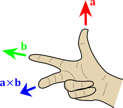
( Modified from http://en.wikipedia.org/wiki/User:Acdx , former image under Creative Commons 3.0 )The X is the notation for the cross product. length( a x b ) == length(a) * length(b) * sin(θ), so you may want to normalize() the result.
Dot product
##
( from http://en.wikipedia.org/wiki/File:Dot_Product.svg )A.B = length(A)cos(Theta) , but most likely computed as A.xB.x +A.yB.y +A.zB.z
Addition and substraction
compontent-wise :
res.x = A.x + B.x
res.y = A.y + B.y
...
Multiplication
compontent-wise :
res.x = A.x * B.x
res.y = A.y * B.y
...
Normalization
Divide the vector by its length :
normalizedVector = vec * ( 1.0f / vec.length() )
Matrices
Matrix-Matrix multiplication
example for a translation matrix :
![]()
Matrix-Vector multiplication
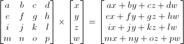
Usual Transformations

… but in your shaders, you can also represent your vectors in tangent space. And in image-space when you do post-effects.
res.x = A.x + B.x
An FPS counter
In real-time graphics, it is important to keep an eye on performance. A good practice is to choose a target FPS ( usually 60 or 30 ) and make everything possible to stick to it.
A FPS counter looks like this :
 double lastTime = glfwGetTime();
 int nbFrames = 0;

 do{

     // Measure speed
     double currentTime = glfwGetTime();
     nbFrames++;
     if ( currentTime - lastTime >= 1.0 ){ // If last prinf() was more than 1 sec ago
         // printf and reset timer
         printf("%f ms/frame\n", 1000.0/double(nbFrames));
         nbFrames = 0;
         lastTime += 1.0;
     }

     ... rest of the main loop
There is an odd thing in this code. It displays the time, in milliseconds, needed to draw a frame (averaged on 1 second) instead of how many frame were drawn in the last second.
This is actually much better. Don’t rely on FPS. Never. FramesPerSecond = 1/SecondsPerFrame, so this is an inverse relationship, and we humans suck at understanding this kind of relationship. Let’s take an example.
You write a great rendering function that runs at 1000 FPS ( 1ms/frame ). But you forgot a little computation in a shader, which adds an extra cost of 0.1ms. And bam, 1/0.0011 = 900. You just lost 100FPS. Morality : never use FPS for performance analysis.
If you intend to make a 60fps game, your target will be 16.6666ms ; If you intend to make a 30fps game, your target will be 33.3333ms. That’s all you need to know.
This code is available in all tutorials starting from Tutorial 9 : VBO indexing; see tutorial09_vbo_indexing/tutorial09.cpp . Other performance tools are available in Tools - Debuggers.
Building your own C application
A lot of efforts have been made so that these tutorials are as simple to compile & run as possible. Unfortunately, this also means that CMakes hides how to do that on your own project.
So, this tutorial will explain how to build your own C application from scatch. But first, you need a basic knowledge of what the compiler actually does.
Please don’t skip the first two sections. If you’re reading this tutorial, you probably need to know this stuff.
The C application model
Preprocessing
This is what all those #defines and #includes are about.
C preprocessing is a very simple process : cut’n pasting.
When the preprocessor sees the following MyCode.c :
#include "MyHeader.h"

void main(){
    FunctionDefinedInHeader();
}
, it simply opens the file MyHeader.h, and cut’n pastes its contents into MyCode.c :
// Begin of MyCode.c
// Begin of MyHeader.h
#ifndef MYHEADER_H
#define MYHEADER_H

void FunctionDefinedInHeader(); // Declare the function

# endif
// End of MyHeader.h

void main(){
    FunctionDefinedInHeader(); // Use it
}

// End of MyCode
Similarly, #defines are cut’n pasted, #ifs are analysed and potentially removed, etc.
At the end of this step we have a preprocessed C++ file, without any #define, #if, #ifdef, #include, ready to be compiled.
As an example, here is the main.cpp file of the 6th tutorial, fully preprocessed in Visual : tutorial06_preprocessed. Warning, it’s a huge file ! But it’s worth knowing what a seemingly simple .cpp really looks to the compiler.
Compilation
The compiler translates C++ code into a representation that the CPU can directly understand. For instance, the following code :
int i=3;
int j=4*i+2;
will be translated into this : x86 opcodes.
mov         dword ptr [i],3
mov         eax,dword ptr [i]
lea         ecx,[eax*4+2]
mov         dword ptr [j],ecx
Each .cpp file is compiled separately, and the resulting binary code is written in .o/.obj files.
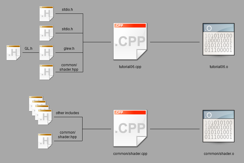
Note that we don’t have an executable yet : one remaining step is needed.
Linking
The linker takes all the binary code (yours, and the one from external libraries), and generates the final executable. A few notes :
- A library has the .lib extension.
- Some libraries are static. This means that the .lib contains all the x86 opcodes needed.
- Some library are dynamic ( also said shared ). This means that the .lib doesn’t contain any x86 code; it simply says “I swear that functions Foo, Bar and WhatsNot will be available at runtime”.
When the linker has run, you have an executable (.exe on Windows, .nothing_at_all on unix) :

Runtime
When you launch the executable, the OS will open the .exe, and put the x86 opcodes in memory. As said earlier, some code isn’t available at this point : the code from dynamic libraries. But the linker was nice enough to say where to look for it : the .exe clearly says that the glClearColor function is implemented in OpenGL32.dll.

Windows will happily open the .dll and find glClearColor :
Sometimes a .dll can’t be found, probably because you screwed the installation process, and the program just can’t be run.
How do I do X with IDE Y ?
The instructions on how to build an OpenGL application are separated from the following basic operations. This is on purpose :
- First, you’ll need to do these thinks all of the time, so you’d better know them well
- Second, you will know what is OpenGL-specific and what is not.
Visual Studio
Creating a new project
File -> New -> Project -> Empty project. Don’t use any weird wizard. Don’t use any option you may not know about (disable MFC, ATL, precompiled headers, stdafx, main file).
Adding a source file in a project
Right clic on Source Files -> Add new.
Adding include directories
Right clic on project -> Project Properties -> C++ -> General -> Additional include directories. This is actually a dropdown list, you can modify the list conveniently.
Link with a library
Right clic on project -> Project Properties -> Linker -> Input -> Additional dependencies : type the name of the .lib. For instance : opengl32.lib
In Project Properties -> Linker -> General -> Additional library directories, make sure that the path to the above library is present.
Build, Run & Debug
Setting the working directory (where your textures & shaders are) : Project Properties -> Debugging -> Working directory
Running : Shift-F5; but you’ll probably never need to do that. Debug instead : F5
A short list of debugging shortcuts :
- F9 on a line, or clicking on the left of the line number: setting a breakpoint. A red dot will appear.
- F10 : execute current line
- F11 : execute current line, but step into the functions this line is calling (“step into”)
- Shift-F11 : run until the end of the function (“step out”)
You also have plenty of debugging windows : watched variables, callstack, threads, …
QtCreator
QtCreator is available for free at http://qt-project.org/.
Creating a new project
Use a plain C or C++ project; avoid the templates filled with Qt stuff.
Use default options.
Adding a source file in a project
Use the GUI, or add the file in the .pro :
SOURCES += main.cpp \
           other.cpp \
           foo.cpp
Adding include directories
In the .pro file :
<code>INCLUDEPATH += <your path> \ <other path> </code>
Link with a library
Right clic on project -> Add library
- If you’re on Linux and you installed the library with apt-get or similar, chances are that the library registered itself in the system. You can select “System package” and enter the name of the library ( ex : libglfw or glew )
- If not, use “System Library”. Browse to where you compiled it.
Build, Run & Debug
Building : Ctrl-B, or the hammer on the bottom left corner.
Running : the green arrow. You can set the program’s arguments and working directory in Projects -> Run Settings
Debugging :
- Setting a breakpoint : Click on the left of the line number. A red dot will appear.
- F10 : execute current line
- F11 : execute current line, but step into the functions this line is calling (“step into”)
- Shift-F11 : run until the end of the function (“step out”)
You also have plenty of debugging windows : watched variables, callstack, threads, …
XCode
Work in progress…
Creating a new project
Adding a source file in a project
Adding include directories
Link with a library
Build, Run & Debug
CMake
CMake will create projects for almost any software building tool : Visual, QtCreator, XCode, make, Code::Blocks, Eclipse, etc, on any OS. This frees you from maintaining many project files.
Creating a new project
Create a CMakeLists.txt file and write the following inside (adapt if needed) :
cmake_minimum_required (VERSION 2.6)
project (your_project_name)

find_package(OpenGL REQUIRED)

add_executable(your_exe_name
    tutorial04_colored_cube/tutorial04.cpp
    common/shader.cpp
    common/shader.hpp
)
Launch the CMake GUI, browse to your .txt file, and select your build folder. Click Configure, then Generate. Your solution will be created in the build folder.
Adding a source file in a project
Simply add a line in the add_executable command.
Adding include directories
include_directories(
    external/AntTweakBar-1.15/include/
    external/glfw-2.7.2/include/
    external/glm-0.9.1/
    external/glew-1.5.8/include/
    .
)
Link with a library
set(ALL_LIBS
    ${OPENGL_LIBRARY}
    GLFW_272
    GLEW_158
    ANTTWEAKBAR_151_OGLCORE_GLFW
)

target_link_libraries(tutorial01_first_window
    ${ALL_LIBS}
)
Build, Run & Debug
CMake doesn’t do that. Use your favourite IDE.
make
Please, just don’t use that.
gcc
It might be worth compiling a small project “by hand” in order to gain a better comprehension of the workflow. Just don’t do this on a real project…
Note that you can also do that on Windows using mingw.
Compile each .cpp file separately :
g++ -c main.cpp
g++ -c tools.cpp
As said above, you will have a main.o and a tools.o files. Link them :
g++ main.o tools.o
a a.out file appeared; It’s your executable, run it :
./a.out
That’s it !
Building your own C application
Armed with this knowledge, we can start building our own OpenGL application.
- Download the dependencies : Here we use GLFW, GLEW and GLM, but depending on your project, you might need something different. Save same preferably in a subdirectory of your project (for instance : external/)
- They should be pre-compiled for your platform. GLM doesn’t have to be compiled, though.
- Create a new project with the IDE of your choice
- Add a new .cpp file in the project
- Copy and paste, for instance, the following code (this is actually playground.cpp) :
#include <stdio.h>
#include <stdlib.h>

#include <GL/glew.h>

#include <GL/glfw.h>

#include <glm/glm.hpp>
using namespace glm;

int main( void )
{
	// Initialise GLFW
	if( !glfwInit() )
	{
		fprintf( stderr, "Failed to initialize GLFW\n" );
		return -1;
	}

	glfwOpenWindowHint(GLFW_FSAA_SAMPLES, 4);
	glfwOpenWindowHint(GLFW_WINDOW_NO_RESIZE,GL_TRUE);
	glfwOpenWindowHint(GLFW_OPENGL_VERSION_MAJOR, 3);
	glfwOpenWindowHint(GLFW_OPENGL_VERSION_MINOR, 3);
	glfwOpenWindowHint(GLFW_OPENGL_PROFILE, GLFW_OPENGL_CORE_PROFILE);

	// Open a window and create its OpenGL context
	if( !glfwOpenWindow( 1024, 768, 0,0,0,0, 32,0, GLFW_WINDOW ) )
	{
		fprintf( stderr, "Failed to open GLFW window. If you have an Intel GPU, they are not 3.3 compatible. Try the 2.1 version of the tutorials.\n" );
		glfwTerminate();
		return -1;
	}

	// Initialize GLEW
	if (glewInit() != GLEW_OK) {
		fprintf(stderr, "Failed to initialize GLEW\n");
		return -1;
	}

	glfwSetWindowTitle( "Playground" );

	// Ensure we can capture the escape key being pressed below
	glfwEnable( GLFW_STICKY_KEYS );

	// Dark blue background
	glClearColor(0.0f, 0.0f, 0.3f, 0.0f);

	do{
		// Draw nothing, see you in tutorial 2 !

		// Swap buffers
		glfwSwapBuffers();

	} // Check if the ESC key was pressed or the window was closed
	while( glfwGetKey( GLFW_KEY_ESC ) != GLFW_PRESS &&
		   glfwGetWindowParam( GLFW_OPENED ) );

	// Close OpenGL window and terminate GLFW
	glfwTerminate();

	return 0;
}
- Compile the project.
You will have many compiler errors. We will analyse all of them, one by one.
Troubleshooting
The error messages below are for Visual Studio 2010, but they are more or less similar on GCC.
Visual Studio - fatal error C1083: Cannot open filetype file: ‘GL/glew.h’ : No such file or directory
(or whichever other file)
Some headers are in weird locations. For instance, GLEW include files are located in external/glew-x.y.z/include/. The compiler has no way to magically guess this, so you have to tell him. In the project settings, add the appropriate path in the COMPILER (not linker) options.
Under no circumstance you should copy files in the compiler’s default directory (Program Files/Visual Studio/…). Technically, this will work, but it’s very bad practice.
Also, it’s good practice to use relative paths ( ./external/glew/… instead of C:/Users/username/Downloads/… )
As an example, this is what the tutorial’s CMake use :
external/glfw-2.7.2/include
external/glm-0.9.1
external/glew-1.5.8/include
Repeat until all files are found.
GCC - fatal error: GL/glew.h: No such file or directory
(or whichever other file)
This means that the library is not installed. If you’re lucky, the library is well-known and you just have to install it. This is the case for GLFW, GLEW and GLM :
sudo apt-get install libglfw-dev libglm-dev libglew1.6-dev
If this is not a widespread library, see the answer for Visual Studio above.
Visual Studio - error LNK2019: unresolved external symbol glfwGetWindowParam referenced in function main
(or whichever other symbol in whichever other function)
Congratulations ! You have a linker error. This is excellent news : this means that the compilation succeeded. Just one last step !
glfw functions are in an external library. You have to tell the linker about this library. Add it in the linker options. Don’t forget to add the path to the library.
As an example, this is what the Visual project use. The names are a bit unusual because this is a custom build. What’s more, GLM doesn’t need to be compiled or linked, so it’s not here.
external\Debug\GLFW_272.lib
external\Debug\GLEW_158.lib
If you download these libraries from SourceForge (GLFW, GLEW) and build a library yourself, you have to specify the correct path. For instance :
C:\Where\You\Put\The\Library\glfw.lib
C:\Where\You\Put\The\Other\Library\glew32.lib
GCC - main.cpp: undefined reference to `glfwInit’
(or whichever other symbol in whichever other file)
Same answer than for Visual Studio.
Note that on Linux, GLFW and GLEW (and many others) are usually installed with apt-get or similar : sudo apt-get install libglew-dev libglfw-dev (may vary). When you do that, the library is copied in the compiler’s standard directory, so you don’t have to specify the path. Just link to glfw and glew as shown in the 1rst section.
I set everything right, but I still have an “unresolved external symbol” error !
This might me tricky to track down. Here are several options:
I have a linker error with _imp_glewInit or some other symbol that begins with _imp
This means that the library (in this case, glew) has been compiled as a static library, but you’re trying to use it as a dynamic library. Simply add the following preprocessor directive in your compiler’s options (for your own project, not glew’s) :
GLEW_STATIC
I have some other weird problem with GLFW
Maybe GLFW was built as a dynamic library, but you’re trying to use it as a static one ?
Try adding the following preprocessor directive :
GLFW_DLL
I have another linker problem ! Help me, I’m stuck !
Please send us a detailed report and a fully featured zipped project, and we’ll add instructions.
I’d like to solve this myself. What are the generic rules ?
Let’s say you’re the author of GLFW. You want to provide the function glfwInit().
When building it as a DLL, you have to tell the compiler that glfwInit() is not like any other function in the DLL : it should be seen from others, unlike glfwPrivateImplementationMethodNobodyShouldCareAbout(). This is done by declaring the function “external” (with GCC) or “__declspec(dllexport)” (with Visual).
When you want to use glfw, you need to tell the compiler that this function is not really available : it should link to it dynamically. This is done by declaring the function “external” (with GCC) or “__declspec(dllimport)” (with Visual).
So you use a handy #define : GLFWAPI, and you use it to declare the functions :
GLFWAPI int glfwInit( void );
- When you’re building as a DLL, you #define GLFW_BUILD_DLL. GLFWAPI then gets #define’d to __declspec(dllexport)
- When you’re using GLFW as a DLL, you #define GLFW_DLL. GLFWAPI then gets #define’d to __declspec(dllimport)
- When you’re building as a static lib, GLFWAPI is #define’d to nothing
- When you’re using GLFW as a static lib, GLFWAPI is #define’d to nothing.
So the rule is : these flags must be consistent. If you build a lib (any lib, not just GLFW) as a DLL, use the right preprocessor definition : GLFW_DLL, GLEW_STATIC
My program crashes !
There are many reasons why a C++ OpenGL application might crash. Here are a few. If you don’t know the exact line where your program crashes, learn how to use a debugger ( see shortcuts above). PLEASE don’t debug with printf().
I don’t even go inside main()
This is most probably because some dll could not be found. Try opening your application with Dependency Walker (Windows) or ldd (Linux; try also this)
My program crashes on glfwOpenWindow(), or any other function that creates an OpenGL context
Several possible reasons :
- Your GPU doesn’t support the requested OpenGL version. Try to see the supported version with GPU Caps Viewer or similar. Update driver if it seems too low. Integrated Intel cards on netbooks especially suck. Use a lower version of OpenGL (2.1 for instance), and use extensions if you lack features.
- Your OS doesn’t support the requested OpenGL version : Mac OS… same answer.
- You’re trying to use GLEW with an OpenGL Core context (i.e. without all the deprecated stuff). This is a GLEW bug. Use glewExperimental=true before glewInit(), or use a compatibility profile ( i.e. use GLFW_OPENGL_COMPAT_PROFILE instead of GLFW_OPENGL_CORE_PROFILE )
My program crashes on the first OpenGL call, or on the first buffer creation
Three possible reasons :
- You’re not calling glewInit() AFTER glfwOpenWindow()
- You’re using a core OpenGL profile, and you didn’t create a VAO. Add the following code after glewInit() :
	GLuint VertexArrayID;
	glGenVertexArrays(1, &VertexArrayID);
	glBindVertexArray(VertexArrayID);
- You’re using the default build of GLEW, which has a bug. You can’t use a Core OpenGL Profile due to this bug. Either Use glewExperimental=true before glewInit(), or ask GLFW for a Compatibility Profile instead :
glfwOpenWindowHint(GLFW_OPENGL_PROFILE, GLFW_OPENGL_COMPAT_PROFILE);
My program crashes when I try to load some file
Setup your working directory correctly. See Tutorial 1.
Create a test.txt file and try the following code :
if ( fopen("test.txt", "r" ) == NULL ){
    printf("I'm probably running my program from a wrong folder");
}
USE THE DEBUGGER !!!! Seriously ! Don’t debug with printf(); use a good IDE. http://www.dotnetperls.com/debugging is for C# but is valid for C++ too. Will vary for XCode and QtCreator, but concepts remain exactly the same.
Something else is wrong
Please contact us by mail
Picking with an OpenGL hack
This technique is not really recommended, but it’s an easy and fast way to add simple picking. By all means, avoid using this in a game, since it might introduce noticeable framerate drops. However, if you have some kind of simulation and you don’t really care about picking performance, this might the perfect option.
Source code for this tutorial is available in misc05_picking/misc05_picking_slow_easy.cpp, which is a quite meaningful name.
Basic idea
The idea behind this technique is to render the scene as usual, but instead of using a nice shading, you render each mesh with a specific and unique color.
Then, you retrieve the colour of the pixel under the mouse cursor and convert this color back to the original identifier. You have your clicked object.
Here’s an example :
In this screenshot, each monkey has a slightly different color, which make is possible to uniquely identify them.
Of course, you don’t want to see the image with all these weird colors, so you also have to clear the screen and re-draw as usual.
Implementation
Giving an ID to every object
Each object of the scene will need a unique color. The easiest way to do this is to give each object an identifying integer, and convert it to a color. This color doesn’t have to have a meaning; this technique is just a hack anyway.
In the accompanying source code, 100 objects are created and stored in a std::vector, so the ID is just the index of the object in the vector. If you have a more complex hierarchy, you’ll probably need to add the ID to your Mesh class, and maintain some sort of std::map to associate the ID with the desired object.
Detecting the click
In this simple example, the picking is done each frame where the left mouse button is down :
if (glfwGetMouseButton(GLFW_MOUSE_BUTTON_LEFT)){
In a real application, you probably want to do this only when the user just released the button, so you’ll have to store a bool wasLeftMouseButtonPressedLastFrame; or, better, use glfwSetMouseButtonCallback() (read GLFW’s manual to know how to use this).
Convert your ID into a special color
Since we’re going to render each mesh with a different color, the first step is to compute this color. An easy way to do this is to put the least signifying bits in the red channels, and the most significant bits in the blue channel :
// Convert "i", the integer mesh ID, into an RGB color
int r = (i & 0x000000FF) >>  0;
int g = (i & 0x0000FF00) >>  8;
int b = (i & 0x00FF0000) >> 16;
This might seem scary, but it’s standard bit-manipulation code. You end up with 3 integers, each in the [0-255] range. With this scheme, you can represent 255^3 = 16 million different meshes, which is probably enough.
Drawing the scene with this color
We now need a shader to use this color. It’s very simple. The vertex shader does nothing :
#version 330 core

// Input vertex data, different for all executions of this shader.
layout(location = 0) in vec3 vertexPosition_modelspace;

// Values that stay constant for the whole mesh.
uniform mat4 MVP;

void main(){

    // Output position of the vertex, in clip space : MVP * position
    gl_Position =  MVP * vec4(vertexPosition_modelspace,1);

}
and the fragment shader simply writes the desired color in the framebuffer :
#version 330 core

// Ouput data
out vec4 color;

// Values that stay constant for the whole mesh.
uniform vec4 PickingColor;

void main(){

    color = PickingColor;

}
Easy !
The only trick is that you have to send your color as floats (in [0,1]) but you have integers (in [0,255]), so you have to make a small division when calling glUniformXX() :
// OpenGL expects colors to be in [0,1], so divide by 255.
glUniform4f(pickingColorID, r/255.0f, g/255.0f, b/255.0f, 1.0f);
You can now draw the meshes as usual (glBindBuffer, glVertexAttribPointer, glDrawElements) and you’ll get the weird picture above.
Get the color under the mouse
When you have drawn all meshes (probably with a for() loop), you need to call glReadPixels(), which will retrieve the rasterized pixels on the CPU. But for this function to work, a few more calls are needed.
First, you need to call glFlush(). This will tell the OpenGL driver to send all the pending commands (including your latest glDrawXX) to the GPU. This is typically not done automatically, because commands are sent in batches, and not immediately (this means that when you call glDrawElements(), nothing is actually draw. It WILL be drawn a few milliseconds later). This operation is SLOW.
Then, you need to call glFinish(), which will wait until everything is really drawn. The difference with glFlush() is that glFlush() just sends the commands; glFinish() waits for these commands to be executed. This operation is SLOOOW.
You also need to configure how glReadPixels will behave with respect to memory alignment. This is a bit off-topic, but you simply need to call glPixelStorei(GL_UNPACK_ALIGNMENT, 1).
And finally, you can call glReadPixels ! Here is the full code :
// Wait until all the pending drawing commands are really done.
// Ultra-mega-over slow !
// There are usually a long time between glDrawElements() and
// all the fragments completely rasterized.
glFlush();
glFinish();
glPixelStorei(GL_UNPACK_ALIGNMENT, 1);
// Read the pixel at the center of the screen.
// You can also use glfwGetMousePos().
// Ultra-mega-over slow too, even for 1 pixel,
// because the framebuffer is on the GPU.
unsigned char data[4];
glReadPixels(1024/2, 768/2,1,1, GL_RGBA, GL_UNSIGNED_BYTE, data);
Your color is now in the ‘data’ array. Here, you can see that the ID is 19.
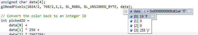
Convert the color back to an ID
You can now reconstruct your ID from the ‘data’ buffer. The code is the complete opposite from the id-to-color code :
// Convert the color back to an integer ID
int pickedID =
data[0] +
data[1] * 256 +
data[2] * 256*256;
Use this ID
You can now use this ID for whatever you need. In the example, the text in the GUI is updated, but of course, you can do whatever you want.
if (pickedID == 0x00ffffff){ // Full white, must be the background !
message = "background";
}else{
std::ostringstream oss; // C++ strings suck
oss << "mesh " << pickedID;
message = oss.str();
}
Pros and cons
Pros :
- Easy, fast to implement
- No need for external library, or complicated math
Cons :
- Use glFlush(), glFinish(), glReadPixels(), all of which are notoriously slow, because they force the CPU to wait for the GPU, which ruins performance.
- You don’t have more precise information : which exact triangle was hit, normal at this point, etc.
Final remarks
While not very recommended, this technique can be really useful; but it’s quite restricted to picking. The methods in the two other tutorials can be used for other purposes, like detecting collisions, making an avatar walk on the ground, visibility queries for AIs, etc.
If you end up using this technique, and you need to pick several points in a single frame, you should do all these points at once. For instance, if you need to handle 5 touch inputs, don’t draw the scene 5 times !
Picking with a physics library
In this tutorial, we will see the “recommended” way to pick objects in a classical game engine - which might not be your case.
The idea is that the game engine will need a physics engine anyway, and all physics engine have functions to intersect a ray with the scene. On top of that, these functions are probably more optimized than what you’ll be able to do yourself : all engines use space partitionning structures, which make it possible to avoid testing intersection with most objects which are not in the same region.
In this tutorial, we will use the Bullet Physics Engine, but the concepts are exactly the same for any other : PhysX, Havok, etc.
Bullet integration
Lots of tutorials explain how to integrate Bullet; in particular, the Bullet’s wiki is very well done.
// Initialize Bullet. This strictly follows http://bulletphysics.org/mediawiki-1.5.8/index.php/Hello_World,
// even though we won't use most of this stuff.
// Build the broadphase
btBroadphaseInterface* broadphase = new btDbvtBroadphase();
// Set up the collision configuration and dispatcher
btDefaultCollisionConfiguration* collisionConfiguration = new btDefaultCollisionConfiguration();
btCollisionDispatcher* dispatcher = new btCollisionDispatcher(collisionConfiguration);
// The actual physics solver
btSequentialImpulseConstraintSolver* solver = new btSequentialImpulseConstraintSolver;
// The world.
btDiscreteDynamicsWorld* dynamicsWorld = new btDiscreteDynamicsWorld(dispatcher,broadphase,solver,collisionConfiguration);
dynamicsWorld->setGravity(btVector3(0,-9.81f,0));
Each object must have a Collision Shape. While this collision shape can be the mesh itself, it’s often a bad idea for performance. Instead, one usually use much simpler shapes as boxes, spheres or capsules. Here are a few collision shapes. From left to right : sphere, cube, convex hull of the mesh, original mesh. Spheres are less precise than the full mesh, but much much faster to test.
In this example, all meshes will use the same box :
btCollisionShape* boxCollisionShape = new btBoxShape(btVector3(1.0f, 1.0f, 1.0f));
Physics engines don’t know anything about OpenGL; and in fact, all of them can run without any 3D visualization at all. So you can’t directly give Bullet your VBO. You have to add a Rigid Body in the simulation instead.
btDefaultMotionState* motionstate = new btDefaultMotionState(btTransform(
btQuaternion(orientations[i].x, orientations[i].y, orientations[i].z, orientations[i].w),
btVector3(positions[i].x, positions[i].y, positions[i].z)
));
btRigidBody::btRigidBodyConstructionInfo rigidBodyCI(
0, // mass, in kg. 0 -> Static object, will never move.
motionstate,
boxCollisionShape, // collision shape of body
btVector3(0,0,0) // local inertia
);
btRigidBody *rigidBody = new btRigidBody(rigidBodyCI);
dynamicsWorld->addRigidBody(rigidBody);
Notice that the Rigid Body use the Collision Shape to determine its shape.
We also keep track of this rigid body, but as the comment says, a real engine would somehow have a MyGameObject class with the position, the orientation, the OpenGL mesh, and a pointer to the Rigid Body.
rigidbodies.push_back(rigidBody);
// Small hack : store the mesh's index "i" in Bullet's User Pointer.
// Will be used to know which object is picked.
// A real program would probably pass a "MyGameObjectPointer" instead.
rigidBody->setUserPointer((void*)i);
In other words : please don’t use the above code in real life ! It’s just for demo purpose.
Raycasting
Finding the ray direction
First, we need to find a ray which starts at the camera and goes “through the mouse”. This is done in the ScreenPosToWorldRay() function.
First, we find the ray’s start and end position in Normalized Device Coordinates. We do it in this space because it’s very easy :
// The ray Start and End positions, in Normalized Device Coordinates (Have you read Tutorial 4 ?)
glm::vec4 lRayStart_NDC(
((float)mouseX/(float)screenWidth - 0.5f) * 2.0f, // [0,1024] -> [-1,1]
((float)mouseY/(float)screenHeight - 0.5f) * 2.0f, // [0, 768] -> [-1,1]
-1.0, // The near plane maps to Z=-1 in Normalized Device Coordinates
1.0f
);
glm::vec4 lRayEnd_NDC(
((float)mouseX/(float)screenWidth - 0.5f) * 2.0f,
((float)mouseY/(float)screenHeight - 0.5f) * 2.0f,
0.0,
1.0f
);
To understand this code, let’s have a look at this picture from Tutorial 4 again :

NDC is a 222 cube centered on the origin, so in this space, the ray going “trough the mouse” is just a straight line, perpendicular to the near plane! Which makes lRayStart_NDC and lEndStart_NDC so easy to compute.
Now we simply have to apply the inverse transformation as the usual one :
// The Projection matrix goes from Camera Space to NDC.
// So inverse(ProjectionMatrix) goes from NDC to Camera Space.
glm::mat4 InverseProjectionMatrix = glm::inverse(ProjectionMatrix);
// The View Matrix goes from World Space to Camera Space.
// So inverse(ViewMatrix) goes from Camera Space to World Space.
glm::mat4 InverseViewMatrix = glm::inverse(ViewMatrix);
glm::vec4 lRayStart_camera = InverseProjectionMatrix * lRayStart_NDC; lRayStart_camera/=lRayStart_camera.w;
glm::vec4 lRayStart_world = InverseViewMatrix * lRayStart_camera; lRayStart_world /=lRayStart_world .w;
glm::vec4 lRayEnd_camera = InverseProjectionMatrix * lRayEnd_NDC; lRayEnd_camera /=lRayEnd_camera .w;
glm::vec4 lRayEnd_world = InverseViewMatrix * lRayEnd_camera; lRayEnd_world /=lRayEnd_world .w;
// Faster way (just one inverse)
//glm::mat4 M = glm::inverse(ProjectionMatrix * ViewMatrix);
//glm::vec4 lRayStart_world = M * lRayStart_NDC; lRayStart_world/=lRayStart_world.w;
//glm::vec4 lRayEnd_world = M * lRayEnd_NDC ; lRayEnd_world /=lRayEnd_world.w;
With lRayStart_worldspace and lRayEnd_worldspace, the ray’s direction (in world space) is straightforward to compute :
glm::vec3 lRayDir_world(lRayEnd_world - lRayStart_world);
lRayDir_world = glm::normalize(lRayDir_world);
Using rayTest()
Raycasting is very simple, no need for special comments :
glm::vec3 out_end = out_origin + out_direction*1000.0f;
btCollisionWorld::ClosestRayResultCallback RayCallback(
btVector3(out_origin.x, out_origin.y, out_origin.z),
btVector3(out_end.x, out_end.y, out_end.z)
);
dynamicsWorld->rayTest(
btVector3(out_origin.x, out_origin.y, out_origin.z),
btVector3(out_end.x, out_end.y, out_end.z),
RayCallback
);
if(RayCallback.hasHit()) {
std::ostringstream oss;
oss << "mesh " << (int)RayCallback.m_collisionObject->getUserPointer();
message = oss.str();
}else{
message = "background";
}
The only thing is that for some weird reason, you have to set the ray’s start and direction twice.
That’s it, you know how to implement picking with Bullet !
Pro and cons
Pros :
- Very easy when you already have a physics engine
- Fast
- Doesn’t impact OpenGL’s performance
Cons :
- Probably not the right solution if you don’t need any physics or collision engine
Final remarks
All physics engines have a debug viewer. The example code shows how to to it with Bullet. You end up with a representation of what Bullet knows about your scene, which is incredibly useful to debug physics-related problem, especially to be sure that the “visual world” is consistent with the “physics world” :

The green box is the Collision Shape, at the same position and orientation than the mesh. The red box is the object’s Axis-Aligned Bounding Box (AABB), which is used as a faster rejection test : if the ray doesn’t intersect the AABB (very cheap to compute), then there is no chance that it will intersect the collision shape. Finally, you can see the object’s axes in blue and red (look at the nose and ear). Handy !
Picking with custom Ray-OBB function
This last method is a nice middleground between the “hacky” pure-OpenGL implementation, and having to integrate a fully-featured physics engine just to do raycasts and picking.
This tutorial uses concepts and functions from the Bullet tutorial, so make sure you read it first.
The basic idea
Instead of relying to Bullet intersect a ray with a Collision Shape, we’re going to do this ourselves.
As we have seen, there are many possible collision shapes. Spheres are very easy to intersect, but for many object, they represent the original mesh very poorly. On the other side, intersecting the ray with each triangle of the original mesh is way to costly. A good middleground are OBB : Oriented Bounding Boxes. There are quite precise (but it depends on your input geometry), and quite cheap to compute.
An OBB is a box that fits the mesh, and when the mesh is translated or rotated, the same transformation is applied to the box :
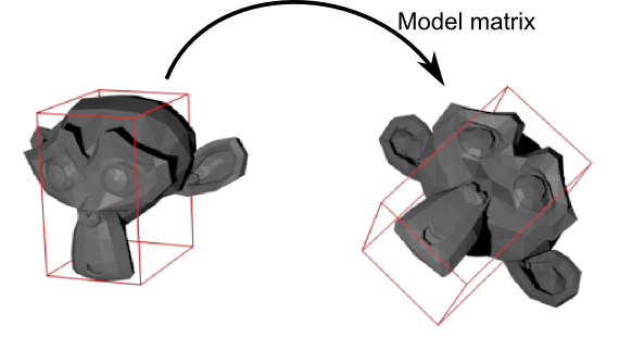
Ray-OBB intersection algorithm
( The algorithm and the pictures are largely inspired from Real-Time Rendering 3. Buy this book ! )
Consider the OBB below. On the X axis, this is delimited by 2 vertical planes, colored in red here. When intersected with the ray (a very simple operation), it gives 2 intersections, one “near” and one “far” :
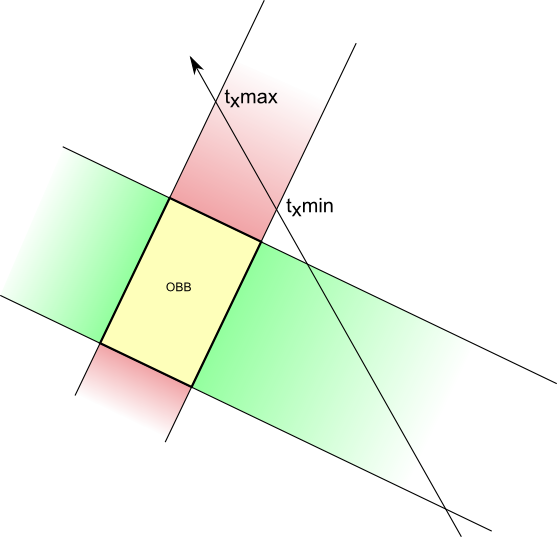
When the ray intersects the 2 others planes that delimit the Y axis (in green), it gives 2 more intersections. Notice how the intersections are ordered : you enter the green area -> you leave the green area -> you enter the red area -> you leave the red area. This means that there is no intersection.

But if this order changes (you enter the green area -> you enter the red area), then you know there is an intersection !
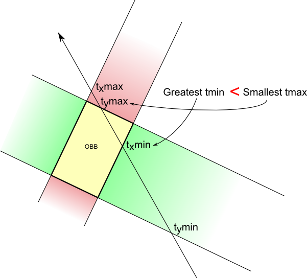
Let’s put this in practice.
Algorithm implementation
(full source code is available in Misc05/misc05_picking_custom.cpp)
Our Ray - OBB intersection function will look like this :
bool TestRayOBBIntersection(
glm::vec3 ray_origin, // Ray origin, in world space
glm::vec3 ray_direction, // Ray direction (NOT target position!), in world space. Must be normalize()'d.
glm::vec3 aabb_min, // Minimum X,Y,Z coords of the mesh when not transformed at all.
glm::vec3 aabb_max, // Maximum X,Y,Z coords. Often aabb_min*-1 if your mesh is centered, but it's not always the case.
glm::mat4 ModelMatrix, // Transformation applied to the mesh (which will thus be also applied to its bounding box)
float& intersection_distance // Output : distance between ray_origin and the intersection with the OBB
){
We begin by nitializing a few variables. tMin is the largest “near” intersection currently found; tMax is the smallest “far” intersection currently found. Delta is used to compute the intersections with the planes.
float tMin = 0.0f;
float tMax = 100000.0f;
glm::vec3 OBBposition_worldspace(ModelMatrix[3].x, ModelMatrix[3].y, ModelMatrix[3].z);
glm::vec3 delta = OBBposition_worldspace - ray_origin;
Now, let’s compute the intersections with the 2 planes that delimit the OBB on the X axis :
glm::vec3 xaxis(ModelMatrix[0].x, ModelMatrix[0].y, ModelMatrix[0].z);
float e = glm::dot(xaxis, delta);
float f = glm::dot(ray_direction, xaxis);
// Beware, don't do the division if f is near 0 ! See full source code for details.
float t1 = (e+aabb_min.x)/f; // Intersection with the "left" plane
float t2 = (e+aabb_max.x)/f; // Intersection with the "right" plane
t1 and t2 now contain distances betwen ray origin and ray-plane intersections, but we don’t know in what order, so we make sure that t1 represents the “near” intersection and t2 the “far” :
if (t1>t2){ // if wrong order
float w=t1;t1=t2;t2=w; // swap t1 and t2
}
We can update tMin and tMax :
// tMax is the nearest "far" intersection (amongst the X,Y and Z planes pairs)
if ( t2 < tMax ) tMax = t2;
// tMin is the farthest "near" intersection (amongst the X,Y and Z planes pairs)
if ( t1 > tMin ) tMin = t1;
And here’s the trick : if “far” is closer than “near”, then there is NO intersection.
if (tMax < tMin )
return false;
This was for the X axis. On all other axes it’s exactly the same !
Using the algorithm
The TestRayOBBIntersection() functions enables us to test the intersection with only one OBB, so we have to test them all. In this tutorial, we simply test all boxes one after the other, but if you have many objects, you might need an additional acceleration structure like a Binary Space Partitionning Tree (BSP-Tree) or a Bounding Volume Hierarchy (BVH).
for(int i=0; i<100; i++){
float intersection_distance; // Output of TestRayOBBIntersection()
glm::vec3 aabb_min(-1.0f, -1.0f, -1.0f);
glm::vec3 aabb_max( 1.0f, 1.0f, 1.0f);
// The ModelMatrix transforms :
// - the mesh to its desired position and orientation
// - but also the AABB (defined with aabb_min and aabb_max) into an OBB
glm::mat4 RotationMatrix = glm::toMat4(orientations[i]);
glm::mat4 TranslationMatrix = translate(mat4(), positions[i]);
glm::mat4 ModelMatrix = TranslationMatrix * RotationMatrix;
if ( TestRayOBBIntersection(
ray_origin,
ray_direction,
aabb_min,
aabb_max,
ModelMatrix,
intersection_distance)
){
std::ostringstream oss;
oss << "mesh " << i;
message = oss.str();
break;
}
}
Note that this algorithm has a problem : it picks the first OBB it finds. But if this OBB is behind another OBB, this is wrong. So you would have to take only the nearest OBB ! Exercise left to the reader…
Pros and cons
Pros :
- Easy
- Low memory requirements (just the OBB’s extents)
- Doesn’t slows OpenGL down as the 1rst version
Cons :
- Slower than a physics engine since there is no acceleration structure
- Might not be precise enough.
Final remarks
There are many other intersection routines available for all sorts of collision shapes; see http://www.realtimerendering.com/intersections.html for instance.
If you need precise intersection, you will have to test ray-triangle intersections. Again, it’s not a good idea to check each triangle of each mesh linearly. Another acceleration structure is required.