Tutorial 16 : Shadow mapping
In Tutorial 15 we learnt how to create lightmaps, which encompasses static lighting. While it produces very nice shadows, it doesn’t deal with animated models.
Shadow maps are the current (as of 2016) way to make dynamic shadows. The great thing about them is that it’s fairly easy to get to work. The bad thing is that it’s terribly difficult to get to work right.
In this tutorial, we’ll first introduce the basic algorithm, see its shortcomings, and then implement some techniques to get better results. Since at time of writing (2012) shadow maps are still a heavily researched topic, we’ll give you some directions to further improve your own shadowmap, depending on your needs.
Basic shadowmap
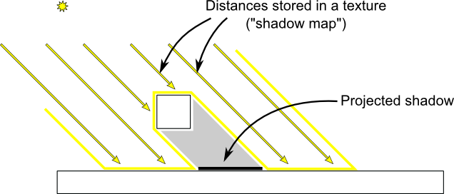
The basic shadowmap algorithm consists in two passes. First, the scene is rendered from the point of view of the light. Only the depth of each fragment is computed. Next, the scene is rendered as usual, but with an extra test to see it the current fragment is in the shadow.
The “being in the shadow” test is actually quite simple. If the current sample is further from the light than the shadowmap at the same point, this means that the scene contains an object that is closer to the light. In other words, the current fragment is in the shadow.
The following image might help you understand the principle :
Rendering the shadow map
In this tutorial, we’ll only consider directional lights - lights that are so far away that all the light rays can be considered parallel. As such, rendering the shadow map is done with an orthographic projection matrix. An orthographic matrix is just like a usual perspective projection matrix, except that no perspective is taken into account - an object will look the same whether it’s far or near the camera.
Setting up the rendertarget and the MVP matrix
Since Tutorial 14, you know how to render the scene into a texture in order to access it later from a shader.
Here we use a 1024x1024 16-bit depth texture to contain the shadow map. 16 bits are usually enough for a shadow map. Feel free to experiment with these values. Note that we use a depth texture, not a depth renderbuffer, since we’ll need to sample it later.
// The framebuffer, which regroups 0, 1, or more textures, and 0 or 1 depth buffer.
 GLuint FramebufferName = 0;
 glGenFramebuffers(1, &FramebufferName);
 glBindFramebuffer(GL_FRAMEBUFFER, FramebufferName);

 // Depth texture. Slower than a depth buffer, but you can sample it later in your shader
 GLuint depthTexture;
 glGenTextures(1, &depthTexture);
 glBindTexture(GL_TEXTURE_2D, depthTexture);
 glTexImage2D(GL_TEXTURE_2D, 0,GL_DEPTH_COMPONENT16, 1024, 1024, 0,GL_DEPTH_COMPONENT, GL_FLOAT, 0);
 glTexParameteri(GL_TEXTURE_2D, GL_TEXTURE_MAG_FILTER, GL_NEAREST);
 glTexParameteri(GL_TEXTURE_2D, GL_TEXTURE_MIN_FILTER, GL_NEAREST);
 glTexParameteri(GL_TEXTURE_2D, GL_TEXTURE_WRAP_S, GL_CLAMP_TO_EDGE);
 glTexParameteri(GL_TEXTURE_2D, GL_TEXTURE_WRAP_T, GL_CLAMP_TO_EDGE);

 glFramebufferTexture(GL_FRAMEBUFFER, GL_DEPTH_ATTACHMENT, depthTexture, 0);

 glDrawBuffer(GL_NONE); // No color buffer is drawn to.

 // Always check that our framebuffer is ok
 if(glCheckFramebufferStatus(GL_FRAMEBUFFER) != GL_FRAMEBUFFER_COMPLETE)
 return false;
The MVP matrix used to render the scene from the light’s point of view is computed as follows :
- The Projection matrix is an orthographic matrix which will encompass everything in the axis-aligned box (-10,10),(-10,10),(-10,20) on the X,Y and Z axes respectively. These values are made so that our entire *visible *scene is always visible ; more on this in the Going Further section.
- The View matrix rotates the world so that in camera space, the light direction is -Z (would you like to re-read Tutorial 3 ?)
- The Model matrix is whatever you want.
glm::vec3 lightInvDir = glm::vec3(0.5f,2,2);

 // Compute the MVP matrix from the light's point of view
 glm::mat4 depthProjectionMatrix = glm::ortho<float>(-10,10,-10,10,-10,20);
 glm::mat4 depthViewMatrix = glm::lookAt(lightInvDir, glm::vec3(0,0,0), glm::vec3(0,1,0));
 glm::mat4 depthModelMatrix = glm::mat4(1.0);
 glm::mat4 depthMVP = depthProjectionMatrix * depthViewMatrix * depthModelMatrix;

 // Send our transformation to the currently bound shader,
 // in the "MVP" uniform
 glUniformMatrix4fv(depthMatrixID, 1, GL_FALSE, &depthMVP[0][0])
The shaders
The shaders used during this pass are very simple. The vertex shader is a pass-through shader which simply compute the vertex’ position in homogeneous coordinates :
#version 330 core

// Input vertex data, different for all executions of this shader.
layout(location = 0) in vec3 vertexPosition_modelspace;

// Values that stay constant for the whole mesh.
uniform mat4 depthMVP;

void main(){
 gl_Position =  depthMVP * vec4(vertexPosition_modelspace,1);
}
The fragment shader is just as simple : it simply writes the depth of the fragment at location 0 (i.e. in our depth texture).
#version 330 core

// Ouput data
layout(location = 0) out float fragmentdepth;

void main(){
    // Not really needed, OpenGL does it anyway
    fragmentdepth = gl_FragCoord.z;
}
Rendering a shadow map is usually more than twice as fast as the normal render, because only low precision depth is written, instead of both the depth and the color; Memory bandwidth is often the biggest performance issue on GPUs.
Result
The resulting texture looks like this :

A dark colour means a small z ; hence, the upper-right corner of the wall is near the camera. At the opposite, white means z=1 (in homogeneous coordinates), so this is very far.
Using the shadow map
Basic shader
Now we go back to our usual shader. For each fragment that we compute, we must test whether it is “behind” the shadow map or not.
To do this, we need to compute the current fragment’s position in the same space that the one we used when creating the shadowmap. So we need to transform it once with the usual MVP matrix, and another time with the depthMVP matrix.
There is a little trick, though. Multiplying the vertex’ position by depthMVP will give homogeneous coordinates, which are in [-1,1] ; but texture sampling must be done in [0,1].
For instance, a fragment in the middle of the screen will be in (0,0) in homogeneous coordinates ; but since it will have to sample the middle of the texture, the UVs will have to be (0.5, 0.5).
This can be fixed by tweaking the fetch coordinates directly in the fragment shader but it’s more efficient to multiply the homogeneous coordinates by the following matrix, which simply divides coordinates by 2 ( the diagonal : [-1,1] -> [-0.5, 0.5] ) and translates them ( the lower row : [-0.5, 0.5] -> [0,1] ).
glm::mat4 biasMatrix(
0.5, 0.0, 0.0, 0.0,
0.0, 0.5, 0.0, 0.0,
0.0, 0.0, 0.5, 0.0,
0.5, 0.5, 0.5, 1.0
);
glm::mat4 depthBiasMVP = biasMatrix*depthMVP;
We can now write our vertex shader. It’s the same as before, but we output 2 positions instead of 1 :
- gl_Position is the position of the vertex as seen from the current camera
- ShadowCoord is the position of the vertex as seen from the last camera (the light)
// Output position of the vertex, in clip space : MVP * position
gl_Position =  MVP * vec4(vertexPosition_modelspace,1);

// Same, but with the light's view matrix
ShadowCoord = DepthBiasMVP * vec4(vertexPosition_modelspace,1);
The fragment shader is then very simple :
- texture( shadowMap, ShadowCoord.xy ).z is the distance between the light and the nearest occluder
- ShadowCoord.z is the distance between the light and the current fragment
… so if the current fragment is further than the nearest occluder, this means we are in the shadow (of said nearest occluder) :
float visibility = 1.0;
if ( texture( shadowMap, ShadowCoord.xy ).z  <  ShadowCoord.z){
    visibility = 0.5;
}
We just have to use this knowledge to modify our shading. Of course, the ambient colour isn’t modified, since its purpose in life is to fake some incoming light even when we’re in the shadow (or everything would be pure black)
color =
 // Ambient : simulates indirect lighting
 MaterialAmbientColor +
 // Diffuse : "color" of the object
 visibility * MaterialDiffuseColor * LightColor * LightPower * cosTheta+
 // Specular : reflective highlight, like a mirror
 visibility * MaterialSpecularColor * LightColor * LightPower * pow(cosAlpha,5);
Result - Shadow acne
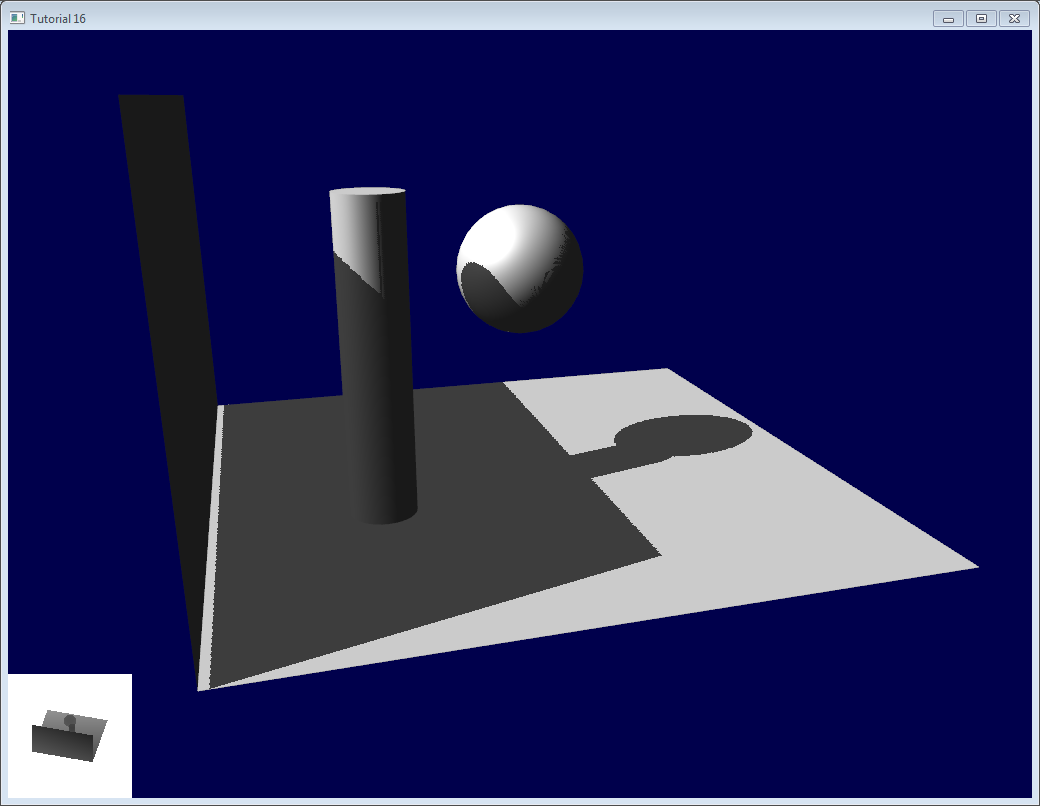
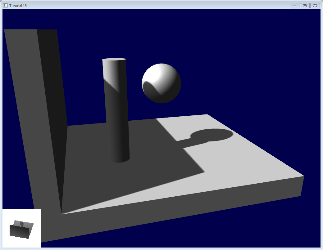
Here’s the result of the current code. Obviously, the global idea it there, but the quality is unacceptable.
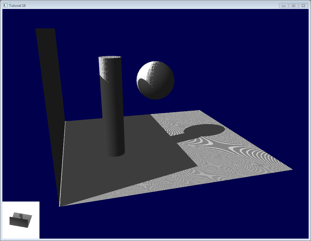
Let’s look at each problem in this image. The code has 2 projects : shadowmaps and shadowmaps_simple; start with whichever you like best. The simple version is just as ugly as the image above, but is simpler to understand.
Problems
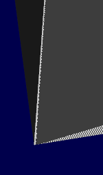
Shadow acne
The most obvious problem is called shadow acne :
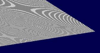
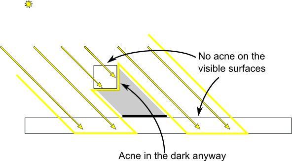
This phenomenon is easily explained with a simple image :
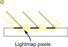
The usual “fix” for this is to add an error margin : we only shade if the current fragment’s depth (again, in light space) is really far away from the lightmap value. We do this by adding a bias :
float bias = 0.005;
float visibility = 1.0;
if ( texture( shadowMap, ShadowCoord.xy ).z  <  ShadowCoord.z-bias){
    visibility = 0.5;
}
The result is already much nicer :
However, you can notice that because of our bias, the artefact between the ground and the wall has gone worse. What’s more, a bias of 0.005 seems too much on the ground, but not enough on curved surface : some artefacts remain on the cylinder and on the sphere.
A common approach is to modify the bias according to the slope :
float bias = 0.005*tan(acos(cosTheta)); // cosTheta is dot( n,l ), clamped between 0 and 1
bias = clamp(bias, 0,0.01);
Shadow acne is now gone, even on curved surfaces.

Another trick, which may or may not work depending on your geometry, is to render only the back faces in the shadow map. This forces us to have a special geometry ( see next section - Peter Panning ) with thick walls, but at least, the acne will be on surfaces which are in the shadow :
When rendering the shadow map, cull front-facing triangles :
        // We don't use bias in the shader, but instead we draw back faces,
        // which are already separated from the front faces by a small distance
        // (if your geometry is made this way)
        glCullFace(GL_FRONT); // Cull front-facing triangles -> draw only back-facing triangles
And when rendering the scene, render normally (backface culling)
glCullFace(GL_BACK); // Cull back-facing triangles -> draw only front-facing triangles
This method is used in the code, in addition to the bias.
Peter Panning
We have no shadow acne anymore, but we still have this wrong shading of the ground, making the wall to look as if it’s flying (hence the term “Peter Panning”). In fact, adding the bias made it worse.
This one is very easy to fix : simply avoid thin geometry. This has two advantages :
- First, it solves Peter Panning : it the geometry is more deep than your bias, you’re all set.
- Second, you can turn on backface culling when rendering the lightmap, because now, there is a polygon of the wall which is facing the light, which will occlude the other side, which wouldn’t be rendered with backface culling.
The drawback is that you have more triangles to render ( two times per frame ! )

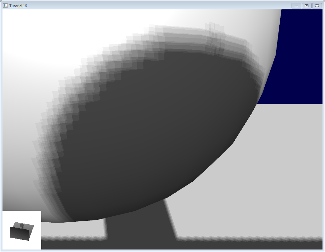
Aliasing
Even with these two tricks, you’ll notice that there is still aliasing on the border of the shadow. In other words, one pixel is white, and the next is black, without a smooth transition inbetween.

PCF
The easiest way to improve this is to change the shadowmap’s sampler type to sampler2DShadow. The consequence is that when you sample the shadowmap once, the hardware will in fact also sample the neighboring texels, do the comparison for all of them, and return a float in [0,1] with a bilinear filtering of the comparison results.
For instance, 0.5 means that 2 samples are in the shadow, and 2 samples are in the light.
Note that it’s not the same than a single sampling of a filtered depth map ! A comparison always returns true or false; PCF gives a interpolation of 4 “true or false”.
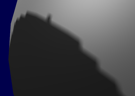
As you can see, shadow borders are smooth, but shadowmap’s texels are still visible.
Poisson Sampling
An easy way to deal with this is to sample the shadowmap N times instead of once. Used in combination with PCF, this can give very good results, even with a small N. Here’s the code for 4 samples :
for (int i=0;i<4;i++){
  if ( texture( shadowMap, ShadowCoord.xy + poissonDisk[i]/700.0 ).z  <  ShadowCoord.z-bias ){
    visibility-=0.2;
  }
}
poissonDisk is a constant array defines for instance as follows :
vec2 poissonDisk[4] = vec2[](
  vec2( -0.94201624, -0.39906216 ),
  vec2( 0.94558609, -0.76890725 ),
  vec2( -0.094184101, -0.92938870 ),
  vec2( 0.34495938, 0.29387760 )
);
This way, depending on how many shadowmap samples will pass, the generated fragment will be more or less dark :
The 700.0 constant defines how much the samples are “spread”. Spread them too little, and you’ll get aliasing again; too much, and you’ll get this :* banding (this screenshot doesn’t use PCF for a more dramatic effect, but uses 16 samples instead) *

Stratified Poisson Sampling
We can remove this banding by choosing different samples for each pixel. There are two main methods : Stratified Poisson or Rotated Poisson. Stratified chooses different samples; Rotated always use the same, but with a random rotation so that they look different. In this tutorial I will only explain the stratified version.
The only difference with the previous version is that we index poissonDisk with a random index :
    for (int i=0;i<4;i++){
        int index = // A random number between 0 and 15, different for each pixel (and each i !)
        visibility -= 0.2*(1.0-texture( shadowMap, vec3(ShadowCoord.xy + poissonDisk[index]/700.0,  (ShadowCoord.z-bias)/ShadowCoord.w) ));
    }
We can generate a random number with a code like this, which returns a random number in [0,1[ :
    float dot_product = dot(seed4, vec4(12.9898,78.233,45.164,94.673));
    return fract(sin(dot_product) * 43758.5453);
In our case, seed4 will be the combination of i (so that we sample at 4 different locations) and … something else. We can use gl_FragCoord ( the pixel’s location on the screen ), or Position_worldspace :
        //  - A random sample, based on the pixel's screen location.
        //    No banding, but the shadow moves with the camera, which looks weird.
        int index = int(16.0*random(gl_FragCoord.xyy, i))%16;
        //  - A random sample, based on the pixel's position in world space.
        //    The position is rounded to the millimeter to avoid too much aliasing
        //int index = int(16.0*random(floor(Position_worldspace.xyz*1000.0), i))%16;
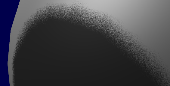
This will make patterns such as in the picture above disappear, at the expense of visual noise. Still, a well-done noise is often less objectionable than these patterns.
See tutorial16/ShadowMapping.fragmentshader for three example implementions.
Going further
Even with all these tricks, there are many, many ways in which our shadows could be improved. Here are the most common :
Early bailing
Instead of taking 16 samples for each fragment (again, it’s a lot), take 4 distant samples. If all of them are in the light or in the shadow, you can probably consider that all 16 samples would have given the same result : bail early. If some are different, you’re probably on a shadow boundary, so the 16 samples are needed.
Spot lights
Dealing with spot lights requires very few changes. The most obvious one is to change the orthographic projection matrix into a perspective projection matrix :
glm::vec3 lightPos(5, 20, 20);
glm::mat4 depthProjectionMatrix = glm::perspective<float>(glm::radians(45.0f), 1.0f, 2.0f, 50.0f);
glm::mat4 depthViewMatrix = glm::lookAt(lightPos, lightPos-lightInvDir, glm::vec3(0,1,0));
same thing, but with a perspective frustum instead of an orthographic frustum. Use texture2Dproj to account for perspective-divide (see footnotes in tutorial 4 - Matrices)
The second step is to take into account the perspective in the shader. (see footnotes in tutorial 4 - Matrices. In a nutshell, a perspective projection matrix actually doesn’t do any perspective at all. This is done by the hardware, by dividing the projected coordinates by w. Here, we emulate the transformation in the shader, so we have to do the perspective-divide ourselves. By the way, an orthographic matrix always generates homogeneous vectors with w=1, which is why they don’t produce any perspective)
Here are two way to do this in GLSL. The second uses the built-in textureProj function, but both methods produce exactly the same result.
if ( texture( shadowMap, (ShadowCoord.xy/ShadowCoord.w) ).z  <  (ShadowCoord.z-bias)/ShadowCoord.w )
if ( textureProj( shadowMap, ShadowCoord.xyw ).z  <  (ShadowCoord.z-bias)/ShadowCoord.w )
Point lights
Same thing, but with depth cubemaps. A cubemap is a set of 6 textures, one on each side of a cube; what’s more, it is not accessed with standard UV coordinates, but with a 3D vector representing a direction.
The depth is stored for all directions in space, which make possible for shadows to be cast all around the point light.
Combination of several lights
The algorithm handles several lights, but keep in mind that each light requires an additional rendering of the scene in order to produce the shadowmap. This will require an enormous amount of memory when applying the shadows, and you might become bandwidth-limited very quickly.
Automatic light frustum
In this tutorial, the light frustum hand-crafted to contain the whole scene. While this works in this restricted example, it should be avoided. If your map is 1Km x 1Km, each texel of your 1024x1024 shadowmap will take 1 square meter; this is lame. The projection matrix of the light should be as tight as possible.
For spot lights, this can be easily changed by tweaking its range.
Directional lights, like the sun, are more tricky : they really do illuminate the whole scene. Here’s a way to compute a the light frustum :
-
Potential Shadow Receivers, or PSRs for short, are objects which belong at the same time to the light frustum, to the view frustum, and to the scene bounding box. As their name suggest, these objects are susceptible to be shadowed : they are visible by the camera and by the light.
-
Potential Shadow Casters, or PCFs, are all the Potential Shadow Receivers, plus all objects which lie between them and the light (an object may not be visible but still cast a visible shadow).
So, to compute the light projection matrix, take all visible objects, remove those which are too far away, and compute their bounding box; Add the objects which lie between this bounding box and the light, and compute the new bounding box (but this time, aligned along the light direction).
Precise computation of these sets involve computing convex hulls intersections, but this method is much easier to implement.
This method will result in popping when objects disappear from the frustum, because the shadowmap resolution will suddenly increase. Cascaded Shadow Maps don’t have this problem, but are harder to implement, and you can still compensate by smoothing the values over time.
Exponential shadow maps
Exponential shadow maps try to limit aliasing by assuming that a fragment which is in the shadow, but near the light surface, is in fact “somewhere in the middle”. This is related to the bias, except that the test isn’t binary anymore : the fragment gets darker and darker when its distance to the lit surface increases.
This is cheating, obviously, and artefacts can appear when two objects overlap.
Light-space perspective Shadow Maps
LiSPSM tweaks the light projection matrix in order to get more precision near the camera. This is especially important in case of “duelling frustra” : you look in a direction, but a spot light “looks” in the opposite direction. You have a lot of shadowmap precision near the light, i.e. far from you, and a low resolution near the camera, where you need it the most.
However LiSPM is tricky to implement. See the references for details on the implementation.
Cascaded shadow maps
CSM deals with the exact same problem than LiSPSM, but in a different way. It simply uses several (2-4) standard shadow maps for different parts of the view frustum. The first one deals with the first meters, so you’ll get great resolution for a quite little zone. The next shadowmap deals with more distant objects. The last shadowmap deals with a big part of the scene, but due tu the perspective, it won’t be more visually important than the nearest zone.
Cascarded shadow maps have, at time of writing (2012), the best complexity/quality ratio. This is the solution of choice in many cases.
Conclusion
As you can see, shadowmaps are a complex subject. Every year, new variations and improvement are published, and to day, no solution is perfect.
Fortunately, most of the presented methods can be mixed together : It’s perfectly possible to have Cascaded Shadow Maps in Light-space Perspective, smoothed with PCF… Try experimenting with all these techniques.
As a conclusion, I’d suggest you to stick to pre-computed lightmaps whenever possible, and to use shadowmaps only for dynamic objects. And make sure that the visual quality of both are equivalent : it’s not good to have a perfect static environment and ugly dynamic shadows, either.